SECTION 5.1 EXERCISES
For Exercise 5.1, see page 283; for Exercise 5.2, see page 284; for Exercise 5.3, see page 286; and for Exercises 5.4 and 5.5, see page 289.
Question 5.6
5.6 Web polls. If you connect to the website peopleschoice.com/pca/polls/polls.jsp, you are given the opportunity to vote on various entertainment questions. Can you apply the ideas about populations and samples to these polls? Explain why or why not.
Question 5.7
5.7 What population and sample? Thirty students from your college who are majoring in English are randomly selected to be on a committee to evaluate immediate changes in the statistics requirement for the major. There are 153 English majors at your college. The current rules say that a statistics course is one of three options for a quantitative competency requirement. The proposed change would be to require a statistics course. Each of the committee members is asked to vote Yes or No on the new requirement.
(a) Describe the population for this setting.
(b) What is the sample?
(c) Describe the statistic and how it would be calculated.
(d) What is the population parameter?
(e) Write a short summary based on your answers to parts (a) through (d) using this setting to explain population, sample, parameter, statistic, and the relationships among these items.
5.7 (a) The population is the 153 English majors at your college. (b) The sample is the 30 selected to be on the committee. (c) The statistic is the number or proportion from the 30 in favor of the change. (d) The parameter would be the number or proportion of all 153 students who would favor the change.
Question 5.8
5.8 What’s wrong? State what is wrong in each of the following scenarios.
(a) A parameter describes a sample.
(b) Bias and variability are two names for the same thing.
(c) Large samples are always better than small samples.
(d) A sampling distribution is something generated by a computer.
Question 5.9
5.9 Describe the population and the sample. For each of the following situations, describe the population and the sample.
(a) A survey of 17,096 students in U.S. four-year colleges reported that 19.4% were binge drinkers.
(b) In a study of work stress, 100 restaurant workers were asked about the impact of work stress on their personal lives.
(c) A tract of forest has 584 longleaf pine trees. The diameters of 40 of these trees were measured.
5.9 (a) Population: all students in the United States at four-year colleges. Sample: the 17,096 students surveyed. (b) Population: all restaurant workers. Sample: the 100 people asked. (c) Population: all 584 longleaf pine trees. Sample: the 40 trees measured.
Question 5.10
5.10 Is it unbiased? A statistic has a sampling distribution that is somewhat skewed. The mean is 17, the median is 15, the quartiles are 13 and 19.
(a) If the population parameter is 15, is the estimator unbiased?
(b) If the population parameter is 17, is the estimator unbiased?
(c) If the population parameter is 16, is the estimator unbiased?
(d) Write a short summary of your results in parts (a), (b), and (c) and include a discussion of bias and unbiased estimators.
Question 5.11
5.11 Constructing a sampling distribution. Refer to Example 5.1 (page 283). Suppose Student Monitor also reported that the median number of hours per week spent on the Internet was 12.5 hours.
(a) Explain why we’d expect the population median to be less than the population mean in this setting by drawing the distribution of times spent on the Internet for all undergraduates. This is called the population distribution.
(b) Using Figure 5.2 (page 285) as a guide and your distribution from part (a), describe how to approximate the sampling distribution of the sample median in this setting.
5.11 (a) We would expect the distribution to be right-skewed, causing the mean to be larger than the median.
Question 5.12
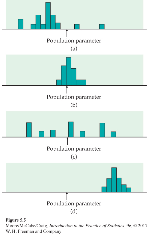
5.12 Bias and variability. Figure 5.5 shows histograms of four sampling distributions of statistics intended to estimate the same parameter. Label each distribution relative to the others as high or low bias and as high or low variability.
Question 5.13
![]() 5.13 Constructing sampling distributions. The Probability applet simulates tossing a coin, with the advantage that you can choose the true long-term proportion, or probability, of a head. Suppose that we have a population in which proportion p = 0.4 (the parameter) plan to vote in the next election. Tossing a coin with probability p = 0.4 of a head simulates this situation: each head is a person who plans to vote, and each tail is a person who does not. Set the “Probability of heads” in the applet to 0.4 and the number of tosses to 25. This simulates an SRS of size 25 from this population. By alternating between “Toss” and “Reset,” you can take many samples quickly.
5.13 Constructing sampling distributions. The Probability applet simulates tossing a coin, with the advantage that you can choose the true long-term proportion, or probability, of a head. Suppose that we have a population in which proportion p = 0.4 (the parameter) plan to vote in the next election. Tossing a coin with probability p = 0.4 of a head simulates this situation: each head is a person who plans to vote, and each tail is a person who does not. Set the “Probability of heads” in the applet to 0.4 and the number of tosses to 25. This simulates an SRS of size 25 from this population. By alternating between “Toss” and “Reset,” you can take many samples quickly.
- Page 292
(a) Take 50 samples, recording the number of heads in each sample. Make a histogram of the 50 sample proportions (count of heads divided by 25). You are constructing the sampling distribution of this statistic.
(b) Another population contains only 20% who plan to vote in the next election. Take 50 samples of size 25 from this population, record the number in each sample who approve, and make a histogram of the 50 sample proportions.
5.13 (a) The shape of the sampling distribution should be roughly Normal centered at 0.4. (b) The shape of the sampling distribution should be roughly Normal centered at 0.2.
Question 5.14
5.14 Comparing sampling distributions. Refer to the previous exercise.
(a) How do the centers of your two histograms reflect the differing truths about the two populations?
(b) Describe any differences in the shapes of the two histograms. Is one more skewed than the other?
(c) Compare the spreads of the two histograms. For which population is there less sampling variability?
(d) Suppose instead that the population proportions were 0.6 and 0.8, respectively. Describe how the sampling distributions of ˆp would differ from those constructed in Exercise 5.13.
Question 5.15
![]() 5.15 Use the Simple Random Sample applet. The Simple Random Sample applet can illustrate the idea of a sampling distribution. Form a population labeled 1 to 100. We will choose an SRS of 15 of these numbers. That is, in this exercise, the numbers themselves are the population, not just labels for 100 individuals. The mean of the whole numbers 1 to 100 is 50.5. This is the parameter, the mean of the population.
5.15 Use the Simple Random Sample applet. The Simple Random Sample applet can illustrate the idea of a sampling distribution. Form a population labeled 1 to 100. We will choose an SRS of 15 of these numbers. That is, in this exercise, the numbers themselves are the population, not just labels for 100 individuals. The mean of the whole numbers 1 to 100 is 50.5. This is the parameter, the mean of the population.
(a) Use the applet to choose an SRS of size 15. Which 15 numbers were chosen? What is their mean? This is a statistic, the sample mean ˉx.
(b) Although the population and its mean 50.5 remain fixed, the sample mean changes as we take more samples. Take another SRS of size 15. (Use the “Reset” button to return to the original population before taking the second sample.) What are the 15 numbers in your sample? What is their mean? This is another value of ˉx.
(c) Take 18 more SRSs from this same population and record their means. You now have 20 values of the sample mean ˉx from 20 SRSs of the same size from the same population. Make a histogram of the 20 values and mark the population mean 50.5 on the horizontal axis. Are your 20 sample values roughly centered at the population value? (If you kept going forever, your ˉx -values would form the sampling distribution of the sample mean; the population mean would indeed be the center of this distribution.)
5.15 (a) and (b) The mean should be “close” to 50.5. (c) The histogram theoretically should be a Normal distribution, centered at 50.5.
Question 5.16
![]() 5.16 Use the Simple Random Sample applet, continued. Refer to the previous exercise.
5.16 Use the Simple Random Sample applet, continued. Refer to the previous exercise.
(a) Suppose instead that a sample size of n = 10 was used. Based on what you know about the effect of the sample size on the sampling distribution, which sampling distribution should have the smaller variability?
(b) Repeat the previous exercise using n = 10. Did your simulations confirm your answer in part (a)? Explain your answer.
(c) Write a short paragraph about the effect of the sample size on the variability of a sampling distribution using these simulations to illustrate the basic idea.