5.3 5.3 Sampling Distributions for Counts and Proportions
When you complete this section, you will be able to:
• Determine when a count X can be modeled using the binomial distribution.
• Determine when the sampling distribution of a count can be modeled using the binomial distribution.
• Calculate the mean and standard deviation of X when it has the B(n, p) distribution.
• Explain the difference between the sampling distribution of a count X and the sampling distribution of the sample proportion ˆp=X/n.
• Determine when one can approximate the sampling distribution of a count using the Normal distribution.
• Determine when one can approximate the sampling distribution of the sample proportion using the Normal distribution.
• Use the Normal approximation for counts and proportions to perform probability calculations about the statistics.
categorical variable, p. 3
In the previous section, we discussed the probability distribution of the sample mean, which meant a focus on population values that were quantitative. We will now shift our focus to population values that are categorical. Counts and proportions are common discrete statistics that describe categorical data.
In Section 5.1 (pages 283–287), we discussed the use of simulation to study the sampling distribution of the sample proportion. In this section, we will use probability theory to more precisely describe the sampling distributions of the sample count and proportion. Let’s start with an example.
EXAMPLE 5.15

Work hours make it difficult to spend time with children. A sample survey asks 1006 British parents whether they think long working hours are making it difficult to spend enough time with their children.11 We would like to view the responses of these parents as representative of a larger population of British parents who hold similar beliefs. That is, we will view the responses of the sampled parents as an SRS from a population.
When there are only two possible outcomes for a random variable, we can summarize the results by giving the count for one of the possible outcomes. We let n represent the sample size, and we use X to represent the random variable that gives the count for the outcome of interest.
EXAMPLE 5.16
The random variable of interest. In this sample survey of British parents, n = 1006. The parents in the sample were asked if they agree with the statement “These days, long working hours make it difficult for parents to spend enough time with their children.” The variable X is the number of parents who agreed with the statement. In this case, X = 755.
In our example, we chose the random variable X to be the number of parents who think that long working hours make it difficult to spend enough time with their children. We could have chosen X to be the number of parents who do not think that long working hours make it difficult to spend enough time with their children. The choice is yours. Often, we make the choice based on how we would like to describe the results in a summary. Which choice do you prefer in this case?
sample proportion, p. 283
When a random variable has only two possible outcomes, it is more common to use the sample proportion ˆp=X/n as the summary rather than the count X.
EXAMPLE 5.17
The sample proportion. The sample proportion of parents surveyed who think that long working hours make it difficult to spend enough time with their children is
ˆp=7551006=0.75
Notice that this summary takes into account the sample size n. We need to know n in order to properly interpret the meaning of the random variable X. For example, the conclusion we would draw about parent opinions in this survey would be quite different if we had observed X = 755 from a sample twice as large, n = 2012.
USE YOUR KNOWLEDGE
Question 5.43
5.43 Sexual harassment in middle school. A survey of 1391 students in grades 5 to 8 reports that 26% of the students say they have encountered some type of sexual harassment while at school.12 Give the sample size n, the count X, and the sample proportion ˆp for this survey.
5.43 n = 1391. X = 362. ˆp=0.26.
Question 5.44
5.44 High school graduates who took a statistics course. In a random sample of n = 4012 high school graduates, 10.8% reported that they had taken a statistics course.13 Give the sample size n, the count X, and the sample proportion ˆp for this setting.
Question 5.45
5.45 Use of the Internet to find a place to live. A poll of 1500 college students asked whether or not they have used the Internet to find a place to live sometime within the past year. There were 1234 students who answered Yes; the other 266 answered No.
(a) What is the sample size n?
(b) Choose one of the two possible outcomes to define the random variable, X. Give a reason for your choice.
(c) What is the value of the count X?
(d) Find the sample proportion, ˆp.
5.45 (a) n = 1500. (c) If the choice is “Yes,” X = 1234. (d) For “Yes,” ˆp=0.8227.
Just like the sample mean, sample counts and sample proportions are commonly used statistics, and understanding their sampling distributions is important for statistical inference. These statistics, however, are discrete random variables, so their sampling distributions introduce us to a new family of probability distributions.
The binomial distributions for sample counts
The distribution of a count X depends on how the data are produced. Here is a simple but common situation.
THE BINOMIAL SETTING
1. There is a fixed number of observations n.
2. The n observations are all independent.
3. Each observation falls into one of just two categories, which for convenience we call “success” and “failure.”
4. The probability of a success, call it p, is the same for each observation.
Think of tossing a coin n times as an example of the binomial setting. Each toss gives either heads or tails, and the outcomes of successive tosses are independent. If we call heads a success, then p is the probability of a head and remains the same as long as we toss the same coin. The number of heads we count is a random variable X. The distribution of X (and, more generally, the distribution of the count of successes in any binomial setting) is completely determined by the number of observations n and the success probability p.
BINOMIAL DISTRIBUTIONS
The distribution of the count X of successes in the binomial setting is called the binomial distribution with parameters n and p. The parameter n is the number of observations, and p is the probability of a success on any one observation. The possible values of X are the whole numbers from 0 to n. As an abbreviation, we say that the distribution of X is B(n, p).
![]()
The binomial distributions are an important class of discrete probability distributions. Later in this section, we will learn how to assign probabilities to outcomes and how to find the mean and standard deviation of binomial distributions. The most important skill for using binomial distributions is the ability to recognize situations to which they do and do not apply. This can be done by checking all the facets of the binomial setting.
EXAMPLE 5.18
Binomial examples? (a) Genetics says that children receive genes from their parents independently. Each child of a particular pair of parents has probability 0.25 of having type O blood. If these parents have three children, the number who have type O blood is the count X of successes in three independent trials with probability 0.25 of a success on each trial. So X has the B(3, 0.25) distribution.
(b) Engineers define reliability as the probability that an item will perform its function under specific conditions for a specific period of time. Replacement heart valves made of animal tissue, for example, have probability 0.77 of performing well for 15 years.14 The probability of failure within 15 years is, therefore, 0.23. It is reasonable to assume that valves in different patients fail (or not) independently of each other. The number of patients in a group of 500 who will need another valve replacement within 15 years has the B(500, 0.23) distribution.
(c) A multicenter trial is designed to assess a new surgical procedure. A total of 540 patients will undergo the procedure, and the count of patients X who suffer a major adverse cardiac event (MACE) within 30 days of surgery will be recorded. Because these patients will receive this procedure from different surgeons at different hospitals, it may not be true that the probability of a MACE is the same for each patient. Thus, X may not have the binomial distribution.
USE YOUR KNOWLEDGE
Question 5.46
5.46 Genetics and blood types. Genetics says that children receive genes from each of their parents independently. Suppose that each child of a particular pair of parents has probability 0.375 of having type AB blood. If these parents have three children, what is the distribution of the number who have type AB blood? Explain your answer.
Question 5.47
5.47 Tossing a coin. Suppose you plan to toss a coin 20 times and record X, the number of heads that you observe. If the coin is fair (p = 0.5), what is the distribution of X? Also, explain why this distribution is also the sampling distribution of X.
5.47 B(20, 0.5).
Binomial distributions in statistical sampling
The binomial distributions are important in statistics when we wish to make inferences about the proportion p of “successes” in a population. Here is a typical example.
EXAMPLE 5.19

Audits of financial records. The financial records of businesses are often audited by state tax authorities to test compliance with tax laws. Suppose that for one retail business, 800 of the 10,000 sales are incorrectly classified as subject to state sales tax. It would be too time-consuming for authorities to examine all these sales. Instead, an auditor examines an SRS of sales records. Is the count X of misclassified records in an SRS of 150 records a binomial random variable?
Choosing an SRS from a population is not quite a binomial setting. Removing one record in Example 5.19 changes the proportion of bad records in the remaining population, so the state of the second record chosen is not independent of the first. Because the population is large, however, removing a few items has a very small effect on the composition of the remaining population. Successive inspection results are very nearly independent. The population proportion of misclassified records is
p=80010,000=0.08
If the first record chosen is bad, the proportion of bad records remaining is 799/9999 = 0.079908. If the first record is good, the proportion of bad records left is 800/9999 = 0.080008. These proportions are so close to 0.08 that, for practical purposes, we can act as if removing one record has no effect on the proportion of misclassified records remaining. We act as if the count X of misclassified sales records in the audit sample has the binomial distribution B(150, 0.08).
stratified random sample, p. 194
Populations like the one described in Example 5.19 often contain a relatively small number of items with very large values. For this example, these values would be very large sale amounts and likely represent an important group of items to the auditor. An SRS taken from such a population will likely include very few items of this type. Therefore, it is common to use a stratified sample in settings like this. Strata are defined based on dollar value of the sale, and within each stratum, an SRS is taken. The results are then combined to obtain an estimate for the entire population.
SAMPLING DISTRIBUTION OF A COUNT
A population contains proportion p of successes. If the population is much larger than the sample, the count X of successes in an SRS of size n has approximately the binomial distribution B(n, p).
The accuracy of this approximation improves as the size of the population increases relative to the size of the sample. As a rule of thumb, we will use the binomial sampling distribution for counts when the population is at least 20 times as large as the sample.
Finding binomial probabilities
We will later give a formula for the probability that a binomial random variable takes any of its values. In practice, you will rarely have to use this formula for calculations because some calculators and most statistical software packages will calculate binomial probabilities for you.
EXAMPLE 5.20
Probabilities for misclassified sales records. In the audit setting of Example 5.19, what is the probability that the audit finds exactly 10 misclassified sales records? What is the probability that the audit finds no more than 10 misclassified records? Figure 5.14 shows the output from one statistical software system. You see that if the count X has the B(150, 0.08) distribution,
P(X = 10) = 0.106959
P(X ≤ 10) = 0.338427
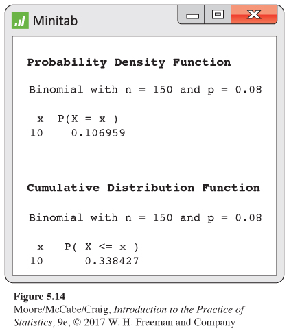
It was easy to request these calculations in the software’s menus. For the TI-83/84 calculator, the functions binompdf and binomcdf would be used. In R, the functions dbinom and pbinom would be used. Typically, the output supplies more decimal places than we need and uses labels that may not be helpful (for example, “Probability Density Function” when the distribution is discrete, not continuous). But, as usual with software, we can ignore distractions and find the results we need.
If you do not have suitable computing facilities, you can still shorten the work of calculating binomial probabilities for some values of n and p by looking up probabilities in Table C in the back of this book. The entries in the table are the probabilities P(X = k) of individual outcomes for a binomial random variable X.
EXAMPLE 5.21
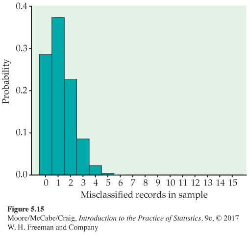
The probability histogram. Suppose that the audit in Example 5.19 chose just 15 sales records. What is the probability that no more than one of the 15 is misclassified? The count X of misclassified records in the sample has approximately the B(15, 0.08) distribution. Figure 5.15 is a probability histogram for this distribution. The distribution is strongly skewed. Although X can take any whole-number value from 0 to 15, the probabilities of values larger than 5 are so small that they do not appear in the histogram.
We want to calculate
| p | ||
| n | k | .08 |
| 15 | 0 | .2863 |
| 1 | .3734 | |
| 2 | .2273 | |
| 3 | .0857 | |
| 4 | .0223 | |
| 5 | .0043 | |
| 6 | .0006 | |
| 7 | .0001 | |
| 8 | ||
| 9 |
P(X ≤ 1) = P(X = 0) + P(X = 1)
when X has the B(15, 0.08) distribution. To use Table C for this calculation, look opposite n = 15 and under p = 0.08. The entries in the rows for each k are P(X = k). Blank cells in the table are 0 to four decimal places. You see that
P(X ≤ 1) = P(X = 0) + P(X = 1)
= 0.2863 + 0.3734 = 0.6597
About two-thirds of all samples will contain no more than one bad record. In fact, almost 29% of the samples will contain no bad records. The sample of size 15 cannot be trusted to provide adequate evidence about misclassified sales records. A larger number of observations is needed.
The values of p that appear in Table C are all 0.5 or smaller. When the probability of a success is greater than 0.5, restate the problem in terms of the number of failures. The probability of a failure is less than 0.5 when the probability of a success exceeds 0.5. When using the table, always stop to ask whether you must count successes or failures.
EXAMPLE 5.22
Falling asleep in class. In the survey of 4513 college students described in Example 5.4, 46% of the respondents reported falling asleep in class due to poor sleep. You randomly sample 10 students in your dormitory, and eight state that they fell asleep in class during the last week due to poor sleep. Relative to the survey results, is this an unusually high number of students?
To answer this question, assume that the students’ actions (falling asleep or not) are independent, with the probability of falling asleep equal to 0.46. This independence assumption may not be reasonable if the students study and socialize together or if there is a loud student in the dormitory who keeps everyone up. We’ll assume this is not an issue here, so the number X of students who fell asleep in class out of 10 students has the B(10, 0.46) distribution.
We want the probability of classifying at least eight students as having fallen asleep in class. Using software, we find
P(X ≥ 8) = P(X = 8) + P(X = 9) + P(X = 10)
= 0.0263 + 0.0050 + 0.0004 = 0.0317
We would expect to find eight or more students falling asleep in class about 3% of the time or in fewer than one of every 30 surveys of 10 students. This is a pretty rare outcome and falls outside the range of the usual chance variation due to random sampling.
USE YOUR KNOWLEDGE
Question 5.48
5.48 Free-throw shooting. April is a college basketball player who makes 80% of her free throws. In a recent game, she had 10 free throws and missed three of them. How unusual is this outcome? Using software, calculator, or Table C, compute 1 − P(X ≤ 2), where X is the number of free throws missed in 10 shots. Explain your answer.
Question 5.49
5.49 Find the probabilities.
(a) Suppose that X has the B(8, 0.3) distribution. Use software, calculator, or Table C to find P(X = 0) and P(X ≥ 6).
(b) Suppose that X has the B(8, 0.7) distribution. Use software, calculator, or Table C to find P(X = 8) and P(X ≤ 2).
(c) Explain the relationship between your answers to parts (a) and (b) of this exercise.
5.49 (a) P(X = 0) = 0.0576 and P(X ≥ 6) = 0.0113. (b) P(X = 8) = 0.0576 and P(X ≤ 2) = 0.0113. (c) The number of “failures” in the B(8, 0.3) distribution has the B(8, 0.3) distribution. With eight trials, zero successes is equivalent to eight failures, and six or more successes is equivalent to two or fewer failures.
Binomial mean and standard deviation
If a count X has the B(n, p) distribution, what are the mean μX and the standard deviation σX? We can guess the mean. If we expect 46% of the students to have fallen asleep in class due to poor sleep, the mean number in 10 students should be 46% of 10, or 4.6. That’s μX when X has the B(10, 0.46) distribution.
Intuition suggests more generally that the mean of the B(n, p) distribution should be np. Can we show that this is correct and also obtain a short formula for the standard deviation? Because binomial distributions are discrete probability distributions, we could find the mean and variance by using the definitions in Section 4.4. Here is an easier way.
A binomial random variable X is the count of successes in n independent observations that each have the same probability p of success. Let the random variable Si indicate whether the ith observation is a success or failure by taking the values Si = 1 if a success occurs and Si = 0 if the outcome is a failure. The Si are independent because the observations are, and each Si has the same simple distribution:
| Outcome | 1 | 0 |
| Probability | p | 1 − p |
From the definition of the mean of a discrete random variable, we know that the mean of each Si is
μS = (1)(p) + (0)(1 − p) = p
Similarly, the definition of the variance shows that σ2S=p(1−p). Because each Si is 1 for a success and 0 for a failure, to find the total number of successes X we add the Si’s:
X = S1 + S2 + · · · + Sn
Apply the addition rules for means and variances to this sum. To find the mean of X we add the means of the Si’s:
μX = μS1 + μS2 + · · · + μSn
= nμS = np
Similarly, the variance is n times the variance of a single S, so that σ2X=np(1−p). The standard deviation σX is the square root of the variance. Here is the result.
BINOMIAL MEAN AND STANDARD DEVIATION
If a count X has the binomial distribution B(n, p), then
μX = np
σX=√np(1−p)
EXAMPLE 5.23
The Helsinki Heart Study. The Helsinki Heart Study asked whether the anticholesterol drug gemfibrozil reduces heart attacks. In planning such an experiment, the researchers must be confident that the sample sizes are large enough to enable them to observe enough heart attacks. The Helsinki study planned to give gemfibrozil to about 2000 men aged 40 to 55 and a placebo to another 2000. The probability of a heart attack during the five-year period of the study for men this age is about 0.04. What are the mean and standard deviation of the number of heart attacks that will be observed in one group if the treatment does not change this probability?
There are 2000 independent observations, each having probability p = 0.04 of a heart attack. The count X of heart attacks has the B(2000, 0.04) distribution, so that
μX = np = (2000)(0.04) = 80
σX=√np(1−p)=√(2000)(0.04)(0.96)=8.76
The expected number of heart attacks is large enough to permit conclusions about the effectiveness of the drug. In fact, there were 84 heart attacks among the 2035 men actually assigned to the placebo, quite close to the mean. The gemfibrozil group of 2046 men suffered only 56 heart attacks. This is evidence that the drug reduces the chance of a heart attack. In a later chapter, we will learn how to determine if this is strong enough evidence to conclude the drug is effective.
USE YOUR KNOWLEDGE
Question 5.50
5.50 Free-throw shooting. Refer to Exercise 5.48. If April takes 85 free throws in the upcoming season, what are the mean and standard deviation of the number of free throws made?
Question 5.51
5.51 Find the mean and standard deviation
(a) Suppose that X has the B(8, 0.3) distribution. Compute the mean and standard deviation of X.
(b) Suppose that X has the B(8, 0.7) distribution. Compute the mean and standard deviation of X.
(c) Explain the relationship between your answers to parts (a) and (b) of this exercise.
5.51 (a) μX = 2.4. σX=1.296. (b) μX = 5.6. σX=1.296. (c) For the means, we have 2.4 + 5.6 = 8. The standard deviations for parts (a) and (b) are the same.
Sample proportions
population proportion, p. 283
What proportion of a company’s sales records have an incorrect sales tax classification? What percent of adults favor stronger laws restricting firearms? In statistical sampling, we often want to estimate the proportion p of “successes” in a population. Our estimator is the sample proportion of successes:
ˆp=count of successes in samplesize of sample=Xn
![]()
Be sure to distinguish between the proportion ˆp and the count X. The count takes whole-number values between 0 and n, but a proportion is always a number between 0 and 1. In the binomial setting, the count X has a binomial distribution. The proportion ˆp does not have a binomial distribution. We can, however, do probability calculations about ˆp by restating them in terms of the count X and using binomial methods. In Example 5.12 (page 303), we took a similar approach for the sum, restating the problem in terms of the sample mean and then using the Normal distribution to calculate the probability.
EXAMPLE 5.24

Shopping online. A survey by the Consumer Reports National Research Center revealed that 84% of all respondents were very satisfied with their online shopping experience.15 It was also reported, however, that people over the age of 40 were generally more satisfied than younger respondents. You decide to take a nationwide random sample of 2500 college students and ask if they agree or disagree that “I am very satisfied with my online shopping experience.” Suppose that 60% of all college students would agree if asked this question. What is the probability that the sample proportion who agree is at least 58%?
The count X who agree has the binomial distribution B(2500, 0.6). The sample proportion ˆp=X/2500 does not have a binomial distribution because it is not a count. But we can translate any question about a sample proportion ˆp into a question about the count X. Because 58% of 2500 is 1450,
P(ˆp ≥ 0.58) = P(X ≥ 1450)
= P(X = 1450) + P(X = 1451) + · · · + P(X = 2500)
This is a rather elaborate calculation. We must add more than 1000 binomial probabilities. Software tells us that P(ˆp≥0.58)=0.9802. But what do we do if we don’t have access to software?
As a first step, find the mean and standard deviation of a sample proportion. We know the mean and standard deviation of a sample count, so apply the rules from Section 4.4 for the mean and variance of a constant times a random variable. Here is the result.
MEAN AND STANDARD DEVIATION OF A SAMPLE PROPORTION
Let ˆp be the sample proportion of successes in an SRS of size n drawn from a large population having population proportion p of successes. The mean and standard deviation of ˆp are
μˆp=pσˆp=√p(1−p)n
The formula for σˆp is exactly correct in the binomial setting. It is approximately correct for an SRS from a large population. We will use it when the population is at least 20 times as large as the sample.
Let’s now use these formulas to calculate the mean and standard deviation for Example 5.24.
EXAMPLE 5.25
The mean and the standard deviation. The mean and standard deviation of the proportion of the survey respondents in Example 5.24 who are satisfied with their online clothes-shopping experience are
μˆp=p=0.6σˆp=√p(1−p)n=√(0.6)(0.4)2500=0.0098
USE YOUR KNOWLEDGE
Question 5.52
5.52 Find the mean and the standard deviation. If we toss a fair coin 150 times, the number of heads is a random variable that is binomial.
(a) Find the mean and the standard deviation of the sample proportion of heads.
(b) Is your answer to part (a) the same as the mean and the standard deviation of the sample count of heads in 150 throws? Explain your answer.
The fact that the mean of ˆp is p states in statistical language that the sample proportion ˆp in an SRS is an unbiased estimator of the population proportion p. When a sample is drawn from a new population having a different value of the population proportion p, the sampling distribution of the unbiased estimator ˆp changes so that its mean moves to the new value of p. We observed this fact empirically in Section 5.1 and have now verified it from the laws of probability.
The variability of ˆp about its mean, as described by the variance or standard deviation, gets smaller as the sample size increases. So a sample proportion from a large sample will usually lie quite close to the population proportion p. We observed this in the simulation experiment on page 285 in Section 5.1. Now we have discovered exactly how the variability decreases: the standard deviation is √p(1−p)/n. Similar to what we observed in the previous section, the √n in the denominator means that the sample size must be multiplied by 4 if we wish to divide the standard deviation in half.
Normal approximation for counts and proportions
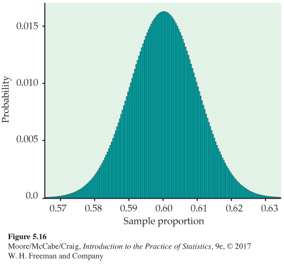
Using simulation, we discovered in Section 5.1 that the sampling distribution of a sample proportion ˆp is close to Normal. Now we know that the distribution of ˆp is that of a binomial count divided by the sample size n. This seems at first to be a contradiction. To clear up the matter, look at Figure 5.16. This is a probability histogram of the exact distribution of the proportion of very satisfied shoppers ˆp, based on the binomial distribution B(2500, 0.6). There are hundreds of narrow bars, one for each of the 2501 possible values of ˆp. Most have probabilities too small to show in a graph. The probability histogram looks very Normal! In fact, both the count X and the sample proportion ˆp are approximately Normal in large samples.
We also know this to be true as a result of the central limit theorem discussed in the previous section (page 298). Recall that we can consider the count X as a sum
X = S1 + S2 + · · · + Sn
of independent random variables Si that take the value 1 if a success occurs on the ith trial and the value 0 otherwise. The proportion of successes ˆp=X/n can then be thought of as the sample mean of the Si and, like all sample means, is approximately Normal when n is large. Given that ˆp is approximately Normal, the count will also be approximately Normal because it is just a constant n times ˆp, an approximately Normal random variable.
NORMAL APPROXIMATION FOR COUNTS AND PROPORTIONS
Draw an SRS of size n from a large population having population proportion p of successes. Let X be the count of successes in the sample and ˆp=X/n be the sample proportion of successes. When n is large, the sampling distributions of these statistics are approximately Normal:
X is approximately N(np,√np(1−p))
ˆp is approximately N(p, √p(1−p)n)
As a rule of thumb, we will use this approximation for values of n and p that satisfy np≥10 and n(1−p)≥10.
These Normal approximations are easy to remember because they say that ˆp and X are Normal, with their usual means and standard deviations. Whether or not you use the Normal approximations should depend on how accurate your calculations need to be. For most statistical purposes, great accuracy is not required. Our “rule of thumb” for use of the Normal approximations reflects this judgment.
![]()
The accuracy of the Normal approximations improves as the sample size n increases. They are most accurate for any fixed n when p is close to 0.5, and least accurate when p is near 0 or 1. You can compare binomial distributions with their Normal approximations by using the Normal Approximation to Binomial applet. This applet allows you to change n or p while watching the effect on the binomial probability histogram and the Normal curve that approximates it.
Figure 5.17 summarizes the distribution of a sample proportion in a form that emphasizes the big idea of a sampling distribution. Just as with Figure 5.11 (page 304), the general framework for constructing a sampling distribution is shown on the left.
• Take many random samples of size n from a population that contains proportion p of successes.
Figure 5.17: Figure 5.17 The sampling distribution of a sample proportion ˆp is approximately Normal with mean p and standard deviation √p(1−p)/n.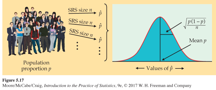 Page 323
• Find the sample proportion ˆp for each sample.
• Collect all the ˆp’s and display their distribution.
The sampling distribution of ˆp is shown on the right. Keep this figure in mind as you move toward statistical inference.
EXAMPLE 5.26
Compare the Normal approximation with the exact calculation. Let’s compare the Normal approximation for the calculation of Example 5.24 with the exact calculation from software. We want to calculate P(ˆp≥0.58) when the sample size is n=2500 and the population proportion is p=0.6. Example 5.25 shows that
μˆp=p=0.6σˆp=√p(1−p)n=0.0098
Act as if ˆp were Normal with mean 0.6 and standard deviation 0.0098. The approximate probability, as illustrated in Figure 5.18, is
P(ˆp≥0.58)=P(ˆp−0.60.0098≥0.58−0.60.0098)
≐ P(Z ≥ −2.04) = 0.9793
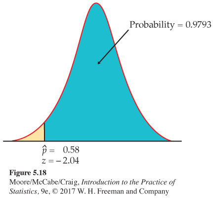
That is, about 98% of all samples have a sample proportion that is at least 0.58. Because the sample was large, this Normal approximation is quite accurate. It misses the software value 0.9802 by only 0.0009.
EXAMPLE 5.27
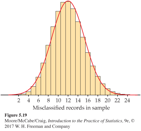
Using the Normal approximation. The audit described in Example 5.19 examined an SRS of 150 sales records for compliance with sales tax laws. In fact, 8% of all the company’s sales records have an incorrect sales tax classification. The count X of bad records in the sample has approximately the B(150, 0.08) distribution.
According to the Normal approximation to the binomial distributions, the count X is approximately Normal with mean and standard deviation
μX=np=(150)(0.08)=12σX=√np(1−p)=√(150)(0.08)(0.92)=3.3226
The Normal approximation for the probability of no more than 10 misclassified records is the area to the left of X = 10 under the Normal curve. Using Table A,
P(X≤10)=P(X−123.3226≤10−123.3226)
≐ P(Z ≤ −0.60) = 0.2743
Software tells us that the actual binomial probability that no more than 10 of the records in the sample are misclassified is P(X≤10)=0.3384. The Normal approximation is only roughly accurate. Because np=12, this combination of n and p is close to the border of the values for which we are willing to use the approximation.
The distribution of the count of bad records in a sample of 15 is distinctly non-Normal, as Figure 5.15 (page 316) showed. When we increase the sample size to 150, however, the shape of the binomial distribution becomes roughly Normal. Figure 5.19 displays the probability histogram of the binomial distribution with the density curve of the approximating Normal distribution superimposed. Both distributions have the same mean and standard deviation, and both the area under the histogram and the area under the curve are 1. The Normal curve fits the histogram reasonably well. Look closely: the histogram is slightly skewed to the right, a property that the symmetric Normal curve can’t match.
USE YOUR KNOWLEDGE
Question 5.53
5.53 Use the Normal approximation. Suppose that we toss a fair coin 150 times. Use the Normal approximation to find the probability that the sample proportion of heads is
(a) between 0.4 and 0.6.
(b) between 0.45 and 0.55.
5.53 (a) 0.9858. (b) 0.7814.
The continuity correction
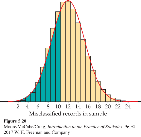
Figure 5.20 illustrates an idea that greatly improves the accuracy of the Normal approximation to binomial probabilities. The binomial probability P(X≤10) is the area of the histogram bars for values 0 to 10. The bar for X=10 actually extends from 9.5 to 10.5. Because the discrete binomial distribution puts probability only on whole numbers, the probabilities P(X≤10) and P(X≤10.5) are the same. The Normal distribution spreads probability continuously, so these two Normal probabilities are different. The Normal approximation is more accurate if we consider X=10 to extend from 9.5 to 10.5, matching the bar in the probability histogram.
The event {X≤10} includes the outcome X=10. Figure 5.20 shades the area under the Normal curve that matches all the histogram bars for outcomes 0 to 10, bounded on the right not by 10, but by 10.5. So P(X≤10) is calculated as P(X≤10.5). On the other hand, P(X<10) excludes the outcome X=10, so we exclude the entire interval from 9.5 to 10.5 and calculate P(X≤9.5) from the Normal table. Here is the result of the Normal calculation in Example 5.27 improved in this way:
P(X≤10)=P(X≤10.5)
=P(X−123.3226≤10.5−123.3226)
≐ P(Z ≤ −0.45) = 0.3264
The improved approximation misses the binomial probability by only 0.012. Acting as though a whole number occupies the interval from 0.5 below to 0.5 above the number is called the continuity correctioncontinuity correction to the Normal approximation. If you need accurate values for binomial probabilities, try to use software to do exact calculations. If no software is available, use the continuity correction unless n is very large. Because most statistical purposes do not require extremely accurate probability calculations, we do not emphasize use of the continuity correction.
Binomial formula
We can find a formula for the probability that a binomial random variable takes any value by adding probabilities for the different ways of getting exactly that many successes in n observations. Here is the example we will use to show the idea.
EXAMPLE 5.28
Blood types of children. Each child born to a particular set of parents has probability 0.25 of having blood type O. If these parents have five children, what is the probability that exactly two of them have type O blood?
The count of children with type O blood is a binomial random variable X with n = 5 tries and probability p = 0.25 of a success on each try. We want P(X = 2).
Because the method doesn’t depend on the specific example, we will use “S” for success and “F” for failure. In Example 5.28, “S” would stand for type O blood. Do the work in two steps.
Step 1: Find the probability that a specific two of the five tries give successes—say, the first and the third. This is the outcome SFSFF. The multiplication rule for independent events tells us that
P(SFSFF) = P(S)P(F)P(S)P(F)P(F)
= (0.25)(0.75)(0.25)(0.75)(0.75)
= (0.25)2(0.75)3
Step 2: Observe that the probability of any one arrangement of two S’s and three F’s has this same probability. That’s true because we multiply together 0.25 twice and 0.75 three times whenever we have two S’s and three F’s. The probability that X = 2 is the probability of getting two S’s and three F’s in any arrangement whatsoever. Here are all the possible arrangements:
SSFFF SFSFF SFFSF SFFFS FSSFF
FSFSF FSFFS FFSSF FFSFS FFFSS
There are 10 of them, all with the same probability. The overall probability of two successes is, therefore,
P(X = 2) = 10(0.25)2(0.75)3 = 0.2637
The pattern of this calculation works for any binomial probability. To use it, we need to be able to count the number of arrangements of k successes in n observations without actually listing them. We use the following fact to do the counting.
BINOMIAL COEFFICIENT
The number of ways of arranging k successes among n observations is given by the binomial coefficient
(nk)=n!k!(n−k)!
for k = 0, 1, 2, . . . , n.
The formula for binomial coefficients uses the factorialfactorial notation. The factorial n! for any positive whole number n is
n! = n × (n − 1) × (n − 2) × · · · × 3 × 2 × 1
Also, 0! = 1. Notice that the larger of the two factorials in the denominator of a binomial coefficient will cancel much of the n! in the numerator. For example, the binomial coefficient we need for Example 5.28 is
(52)=5!2!3!=(5)(4)(3)(2)(1)(2)(1)×(3)(2)(1)=(5)(4)(2)(1)=202=10
This agrees with our previous calculation.
![]()
The notation (nk) is not related to the fraction nk. A helpful way to remember its meaning is to read it as “binomial coefficient n choose k.” Binomial coefficients have many uses in mathematics, but we are interested in them only as an aid to finding binomial probabilities. The binomial coefficient (nk) counts the number of ways in which k successes can be distributed among n observations. The binomial probability P(X=k) is this count multiplied by the probability of any specific arrangement of the k successes. Here is the formula we seek.
BINOMIAL PROBABILITY
If X has the binomial distribution B(n, p) with n observations and probability p of success on each observation, the possible values of X are 0, 1, 2, . . . , n. If k is any one of these values, the binomial probability is
P(X=k)=(nk)pk(1−p)n−k
Here is an example of the use of the binomial probability formula.
EXAMPLE 5.29
Using the binomial probability formula. The number X of misclassified sales records in the auditor’s sample in Example 5.21 (page 316) has the B(15,0.08) distribution. The probability of finding no more than one misclassified record is
P(X≤1)=P(X=0)+P(X=1)=(150)(0.08)0(0.92)15+(151)(0.08)1(0.92)14=15!0!15!(1)(0.2863)+15!1!14!(0.08)(0.3112)=(1)(1)(0.2863)+(15)(0.08)(0.3112)=0.2863+0.3734=0.6597
The calculation used the facts that 0! = 1 and that a0=1 for any number a≠0. The result agrees with that obtained from Table C in Example 5.21.
USE YOUR KNOWLEDGE
Question 5.54
5.54 An unfair coin. A coin is slightly bent, and as a result, the probability of a head is 0.53. Suppose that you toss the coin five times.
(a) Use the binomial formula to find the probability of three or more heads.
(b) Compare your answer with the one that you would obtain if the coin were fair.
The Poisson distributions
A count X has a binomial distribution when it is produced under the binomial setting. If one or more facets of this setting do not hold, the count X will have a different distribution. In this subsection, we discuss one of these distributions.
Frequently, we meet counts that are open-ended; that is, they are not based on a fixed number of n observations: the number of customers at a popular café between 12:00 P.M. and 1:00 P.M.; the number of dings on your car door; the number of reported pedestrian/bicyclist collisions on campus during the academic year. These are all counts that could be 0, 1, 2, 3, and so on indefinitely.
The Poisson distribution is another model for a count and can often be used in these open-ended situations. The count represents the number of events (call them “successes”) that occur in some fixed unit of measure such as a period of time or region of space. The Poisson distribution is appropriate under the following conditions.
THE POISSON SETTING
1. The number of successes that occur in two nonoverlapping units of measure are independent.
2. The probability that a success will occur in a unit of measure is the same for all units of equal size and is proportional to the size of the unit.
3. The probability that more than one event occurs in a unit of measure is negligible for very small-sized units. In other words, the events occur one at a time.
For binomial distributions, the important quantities were n, the fixed number of observations, and p, the probability of success on any given observation. For Poisson distributions, the only important quantity is the mean number of successes μ occurring per unit of measure.
POISSON DISTRIBUTION
The distribution of the count X of successes in the Poisson setting is the Poisson distribution with mean μ. The parameter μ is the mean number of successes per unit of measure. The possible values of X are the whole numbers 0, 1, 2, 3, . . . . If k is any whole number, then*
P(X=k)=e−μμkk!
The standard deviation of the distribution is √μ.
EXAMPLE 5.30
Number of dropped calls. Suppose that the number of dropped calls on your cell phone varies, with an average of 2.1 calls per day. If we assume that the Poisson setting is reasonable for this situation, we can model the daily count of dropped calls X using the Poisson distribution with μ=2.1. What is the probability of having no more than two dropped calls tomorrow?
We can calculate P(X≤2) either using software or the Poisson probability formula. Using the probability formula:
P(X≤2)=P(X=0)+P(X=1)+P(X=2)
=e−2.1(2.1)00!+e−2.1(2.1)11!+e−2.1(2.1)22!
= 0.1225 + 0.2572 + 0.2700
= 0.6497
Using the R software, the probability is
dpois(0,2.1)+dpois(1,2.1)+dpois(2,2.1)[1] 0.6496314
These two answers differ slightly due to roundoff error in the hand calculation. There is roughly a 65% chance that you will have no more than two dropped calls tomorrow.
Similar to the binomial, Poisson probability calculations are rarely done by hand if the event includes numerous possible values for X. Most software provides functions to calculate P(X=k) and the cumulative probabilities of the form P(X≤k). These cumulative probability calculations make solving many problems less tedious. Here’s an example.
EXAMPLE 5.31
Counting software remote users. Your university supplies online remote access to various software programs used in courses. Suppose that the number of students remotely accessing these programs in any given hour can be modeled by a Poisson distribution with μ=17.2. What is the probability that more than 25 students will remotely access these programs in the next hour?
Calculating this probability requires two steps.
1. Write P(X>25) as an expression involving a cumulative probability:
P(X>25)=1−P(X≤25)
2. Obtain P(X≤25) and subtract the value from 1. Again using R,
1- ppois(25,17.2)[1] 0.02847261
The probability that more than 25 students will use this remote access in the next hour is only 0.028. Relying on software to get the cumulative probability is much quicker and less prone to error than the method of Example 5.30. For this case, that method would involve determining 26 probabilities and then summing their values.
Under the Poisson setting, this probability of 0.028 applies not only to the next hour, but also to any other hour in the future. The probability does not change because the units of measure are the same size and nonoverlapping.
USE YOUR KNOWLEDGE
Question 5.55
5.55 Number of aphids. The milkweed aphid is a common pest to many ornamental plants. Suppose that the number of aphids on a shoot of a Mexican butterfly weed follows a Poisson distribution with μ = 4.4 aphids.
(a) What is the probability of observing exactly five aphids on a shoot?
(b) What is the probability of observing five or fewer aphids on a shoot?
5.55 (a) 0.1687. (b) 0.7199.
Question 5.56
5.56 Number of aphids, continued. Refer to the previous exercise.
(a) What proportion of shoots would you expect to have no aphids present?
(b) If you do not observe any aphids on a shoot, is the probability that a nearby shoot has no aphids smaller than, equal to, or larger than your answer in part (a)? Explain your reasoning.
If we add counts from successive nonoverlapping areas of equal size, we are just counting the successes in a larger area. That count still meets the conditions of the Poisson setting. However, because our unit of measure has doubled, the mean of this new count is twice as large. Put more formally, if X is a Poisson random variable with mean μX and Y is a Poisson random variable with mean μY and Y is independent of X, then X+Y is a Poisson random variable with mean μX+μY. This fact means that we can combine areas or look at a portion of an area and still use Poisson distributions to model the count.
EXAMPLE 5.32
Number of potholes. The Automobile Association (AA) in Britain had member volunteers make a 60-minute, two-mile walk around their neighborhoods and survey the condition of their roads and sidewalks. One outcome was the number of potholes, defined as being at least 2 inches deep and at least 6 inches in diameter, in their roads.16 It was reported that Scotland averages 8.9 potholes per mile of road and London averages 4.9 potholes per mile of road. Suppose that the number of potholes per mile in each of these two regions follow the Poisson distribution. Then
• The number of potholes per 20 miles of road in Scotland is a Poisson random variable with mean 20×8.9=178.
• The number of potholes per half mile of road in London is a Poisson random variable with mean 0.5×4.9=2.45.
• The number of potholes per 500 miles of road in Scotland is a Poisson random variable with mean 500×8.9=4450.
• If we examined 2 miles of road in Scotland and 5 miles of road in London, the total number of potholes would be a Poisson random variable with mean 2×8.9+5×4.9=42.3.
When the mean of the Poisson distribution is large, it may be difficult to calculate Poisson probabilities using a calculator or software. Fortunately, when μ is large, Poisson probabilities can be approximated using the Normal distribution with mean μ and standard deviation √μ. Here is an example.
EXAMPLE 5.33
Number of snaps received. In Example 5.11, it was reported that Snapchat has more than 100 million daily users who send over 400 million snaps a day. Suppose that the number of snaps you receive per day follows a Poisson distribution with mean 12. What is the probability that, over a week, you would receive more than 100 snaps?
To answer this using software, we first compute the mean number of snaps sent per week. Because there are seven days in a week, the mean is 7×12=84. Plugging this into R tells us that there is slightly less than an 4% chance of receiving this many snaps:
1-ppois(100,84)[1] 0.03891883
For the Normal approximation we compute
P(X>100)=P(X−84√84>100−84√84)=P(Z>1.75)=1−P(Z<1.75)=1−0.9599=0.0401
The approximation is quite accurate, differing from the actual probability by only 0.0012.
While the Normal approximation is adequate for many practical purposes, we recommend using statistical software when possible so you can get exact Poisson probabilities.
There is one other approximation associated with the Poisson distribution that is worth mentioning. It is related to the binomial distribution. Previously, we recommended using the Normal distribution to approximate the binomial distribution when n and p satisfy np≥10 and n(1−p)≥10. In cases where n is large but p is so small that np<10, the Poisson distribution with μ=np yields more accurate results. For example, suppose that you wanted to calculate P(X≤2) when X has the B(1000, .001) distribution. Using R, the actual binomial probability and the Poisson approximation are
pbinom(2, 1000,.001)ppois(2, 1)[1] 0.9197907[1] 0.9196986
The Poisson approximation gives a very accurate probability calculation for the binomial distribution in this case.