6.4 6.4 Power and Inference as a Decision
When you complete this section, you will be able to:
• Define what is meant by the power of a test.
• Determine the power of a test to detect an alternative for a given sample size n.
• Describe the two types of possible errors when performing a test that focuses on deciding between two hypotheses.
• Relate the two errors to the significance level and power of the test.
Although we prefer to use P-values rather than the reject-or-not view of the level α significance test, the latter view is very important for planning studies and for understanding statistical decision theory. We will discuss these two topics in this section.
Power
Level α significance tests are closely related to confidence intervals—in fact, we saw that a two-sided test can be carried out directly from a confidence interval (pages 353–354). The significance level, like the confidence level, says how reliable the method is in repeated use. If we use 5% significance tests repeatedly when H0 is, in fact, true, we will be wrong (the test will reject H0) 5% of the time and right (the test will fail to reject H0) 95% of the time.
The ability of a test to detect that H0 is false is measured by the probability that the test will reject H0 when an alternative is true. The higher this probability is, the more sensitive the test is.
POWER
The probability that a level α significance test will reject H0 when a particular alternative value of the parameter is true is called the power of the test to detect that alternative.
EXAMPLE 6.29
The power of a TBBMC significance test. Can a six-month exercise program increase the total body bone mineral content (TBBMC) of young women? A team of researchers is planning a study to examine this question. Based on the results of a previous study, they are willing to assume that σ = 2 for the percent change in TBBMC over the six-month period. They also believe that a change in TBBMC of 1% is important, so they would like to have a reasonable chance of detecting a change this large or larger. Is 25 subjects a large enough sample for this project?
We will answer this question by calculating the power of the significance test that will be used to evaluate the data to be collected. The calculation consists of three steps:
1. State H0, Ha (the particular alternative we want to detect), and the significance level α.
2. Find the values of ˉx that will lead us to reject H0.
3. Calculate the probability of observing these values of ˉx when the alternative is true.
Step 1. The null hypothesis is that the exercise program has no effect on TBBMC. In other words, the mean percent change is zero. The alternative is that exercise is beneficial; that is, the mean change is positive. Formally, we have
H0: μ = 0
Ha: μ > 0
The alternative of interest is μ = 1% increase in TBBMC. A 5% test of significance will be used.
Step 2. The z test rejects H0 at the α = 0.05 level whenever
z=ˉx−μ0σ/√n=ˉx−02/√25≥1.645
Be sure you understand why we use 1.645. Rewrite this in terms of ˉx:
ˉx≥1.6452√25ˉx≥0.658
Because the significance level is α = 0.05, this event has probability 0.05 of occurring when the population mean μ is 0.
Step 3. The power to detect the alternative μ = 1% is the probability that H0 will be rejected when in fact μ = 1%. We calculate this probability by standardizing ˉx, using the value μ = 1, the population standard deviation σ = 2, and the sample size n = 25. The power is
P(ˉx≥0.658 when μ=1)=P(ˉx−μσ/√n≥0.658−12/√25)
= P(Z ≥ −0.855) = 0.80
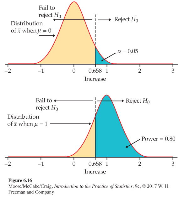
Figure 6.16 illustrates the power with the sampling distribution of ˉx when μ = 1. This significance test rejects the null hypothesis that exercise has no effect on TBBMC 80% of the time if the true effect of exercise is a 1% increase in TBBMC. If the true effect of exercise is a greater percent increase, the test will have greater power; it will reject with a higher probability.
Here is another example of a power calculation, this time for a two-sided z test.
EXAMPLE 6.30
Power of the lead concentration test. Example 6.17 (page 375) presented a test of
H0: μ = 15.00
Ha: μ ≠ 15.00
at the 1% level of significance. What is the power of this test against the specific alternative μ = 15.50?
The test rejects H0 when |z| ≥ 2.576. The test statistic is
z=ˉx−15.000.25/√3
Some arithmetic shows that the test rejects when either of the following is true:
z ≥ 2.576 (in other words, ˉx ≥ 15.37)
z ≤ −2.576 (in other words, ˉx ≤ 14.63)
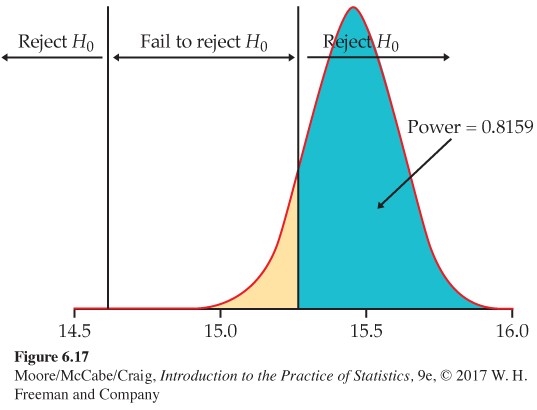
These are disjoint events, so the power is the sum of their probabilities, computed assuming that the alternative μ = 15.50 is true. We find that
P(ˉx≥15.37)=P(ˉx−μσ/√n≥15.37−15.500.25/√3)
= P(Z ≥ −0.90) = 0.8159
P(ˉx≤14.63)=P(ˉx−μσ/√n≤14.63−15.500.25/√3)
= P(Z ≤ −6.03) ≐ 0
Figure 6.17 illustrates this calculation. A power of about 0.82, we are quite confident that the test will reject H0 when this alternative is true.
High power is desirable. Along with 95% confidence intervals and 5% significance tests, 80% power is becoming a standard. Many U.S. government agencies that provide research funds require that the sample size for the funded studies be sufficient to detect important results 80% of the time using a 5% test of significance.
EXAMPLE 6.31
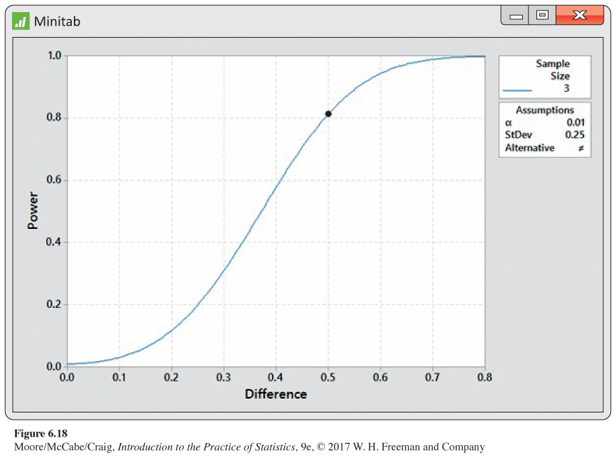
Constructing a power curve. Example 6.30 considered one specific alternative, μ = 15.50. Often, it is helpful to consider the power for a range of alternatives. Fortunately, most statistical software saves us from having to do these calculations manually. Figure 6.18 shows Minitab output for the power over the range 15.00 ppm to 15.80 ppm. The power calculation of Example 6.30 is represented by a dot on the curve at a difference of 15.50 − 15.00 = 0.50. This curve is very informative. We see that with a sample size of three, the power is greater than 80% only for differences larger than about 0.48. If it is important to detect differences less than this, the Deely Laboratory needs to consider ways to increase the power.
Increasing the power
Suppose that you have performed a power calculation and found that the power is too small. What can you do to increase it? Here are four ways. Note the similarity between these and the choices to reduce the margin of error (page 352).
• Increase α. A 5% test of significance will have a greater chance of rejecting the alternative than a 1% test because the strength of evidence required for rejection is less.
• Consider a particular alternative that is farther away from μ0. Values of μ that are in Ha but lie close to the hypothesized value μ0 are harder to detect (lower power) than values of μ that are far from μ0.
• Increase the sample size. More data will provide more information about ˉx so we have a better chance of distinguishing values of μ.
• Decrease σ. This has the same effect as increasing the sample size: more information about μ. Improving the measurement process and restricting attention to a subpopulation are possible ways to decrease σ.
Power calculations are important in planning studies. Using a significance test with low power makes it unlikely that you will find a significant effect even if the truth is far from the null hypothesis. A null hypothesis that is, in fact, false can become widely believed if repeated attempts to find evidence against it fail because of low power. The following example illustrates this point.
EXAMPLE 6.32
Are stock markets efficient? The “efficient market hypothesis” for the time series of stock prices says that future stock prices (when adjusted for inflation) show only random variation. No information available now will help us predict stock prices in the future because the efficient working of the market has already incorporated all available information in the present price. Many studies have tested the claim that one or another kind of information is helpful. In these studies, the efficient market hypothesis is H0, and the claim that prediction is possible is Ha. Almost all the studies have failed to find good evidence against H0. As a result, the efficient market hypothesis is quite popular. But an examination of the significance tests employed finds that the power is generally low. Failure to reject H0 when using tests of low power is not evidence that H0 is true. As one expert says, “The widespread impression that there is strong evidence for market efficiency may be due just to a lack of appreciation of the low power of many statistical tests.”30
Inference as decision
We have presented tests of significance as methods for assessing the strength of evidence against the null hypothesis. This assessment is made by the P-value, which is a probability computed under the assumption that H0 is true. The alternative hypothesis (the statement we seek evidence for) enters the test only to help us see what outcomes count against the null hypothesis.
There is another way to think about these issues. Sometimes, we are really concerned about making a decision or choosing an action based on our evaluation of the data. Acceptance samplingacceptance sampling is one such circumstance. A producer of bearings and a skateboard manufacturer agree that each carload lot of bearings shall meet certain quality standards. When a carload arrives, the manufacturer chooses a sample of bearings to be inspected. On the basis of the sample outcome, the manufacturer will either accept or reject the carload. Let’s examine how the idea of inference as a decision changes the reasoning used in tests of significance.
Two types of error
Tests of significance concentrate on H0, the null hypothesis. If a decision is called for, however, there is no reason to single out H0. There are simply two hypotheses, and we must accept one and reject the other. It is convenient to call the two hypotheses H0 and Ha, but H0 no longer has the special status (the statement we try to find evidence against) that it had in tests of significance. In the acceptance sampling problem, we must decide between
H0: the lot of bearings meets standards
Ha: the lot does not meet standards
on the basis of a sample of bearings.
We hope that our decision will be correct, but sometimes it will be wrong. There are two types of incorrect decisions. We can accept a bad lot of bearings, or we can reject a good lot. Accepting a bad lot injures the consumer, while rejecting a good lot hurts the producer. To help distinguish these two types of error, we give them specific names.
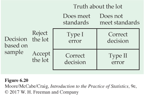
TYPE I AND TYPE II ERRORS
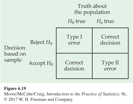
If we reject H0 (accept Ha) when in fact H0 is true, this is a Type I error. If we accept H0 (reject Ha) when in fact Ha is true, this is a Type II error.
The possibilities are summed up in Figure 6.19. If H0 is true, our decision either is correct (if we accept H0) or is a Type I error. If Ha is true, our decision either is correct or is a Type II error. Only one error is possible at one time. Figure 6.20 applies these ideas to the acceptance sampling example.
Error probabilities
Any rule for making decisions is assessed in terms of the probabilities of the two types of error. This is in keeping with the idea that statistical inference is based on probability. We cannot (short of inspecting the whole lot) guarantee that good lots of bearings will never be rejected and bad lots never be accepted. But by random sampling and the laws of probability, we can say what the probabilities of both kinds of error are.
Significance tests with fixed level α give a rule for making decisions because the test either rejects H0 or fails to reject it. If we adopt the decision-making way of thought, failing to reject H0 means deciding that H0 is true. We can then describe the performance of a test by the probabilities of Type I and Type II errors.
EXAMPLE 6.33

Outer diameter of a skateboard bearing. The mean outer diameter of a skateboard bearing is supposed to be 22.000 millimeters (mm). The outer diameters vary Normally with standard deviation σ = 0.010 mm. When a lot of the bearings arrives, the skateboard manufacturer takes an SRS of five bearings from the lot and measures their outer diameters. The manufacturer rejects the bearings if the sample mean diameter is significantly different from 22 mm at the 5% significance level.
This is a test of the hypotheses
H0: μ = 22
Ha: μ ≠ 22
To carry out the test, the manufacturer computes the z statistic:
z=ˉx−220.01/√5
and rejects H0 if
z < −1.96 or z > 1.96
A Type I error is to reject H0 when in fact μ = 22.
What about Type II errors? Because there are many values of μ in Ha, we will concentrate on one value. The producer and the manufacturer agree that a lot of bearings with mean 0.015 mm away from the desired mean 22.000 should be rejected. So a particular Type II error is to accept H0 when in fact μ = 22.015.
Figure 6.21 shows how the two probabilities of error are obtained from the two sampling distributions of ˉx, for μ = 22 and for μ = 22.015. When μ = 22, H0 is true and to reject H0 is a Type I error. When μ = 22.015, accepting H0 is a Type II error. We will now calculate these error probabilities.
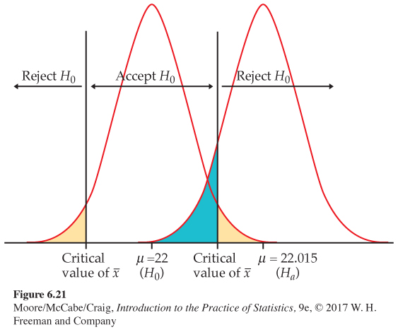
The probability of a Type I error is the probability of rejecting H0 when it is really true. In Example 6.33, this is the probability that |z| ≥ 1.96 when μ = 22. But this is exactly the significance level of the test. The critical value 1.96 was chosen to make this probability 0.05, so we do not have to compute it again. The definition of “significant at level 0.05” is that sample outcomes this extreme will occur with probability 0.05 when H0 is true.
SIGNIFICANCE AND TYPE I ERROR
The significance level α of any fixed level test is the probability of a Type I error. That is, α is the probability that the test will reject the null hypothesis H0 when H0 is in fact true.
The probability of a Type II error for the particular alternative μ = 22.015 in Example 6.33 is the probability that the test will fail to reject H0 when μ has this alternative value. The power of the test to detect the alternative μ = 22.015 is just the probability that the test does reject H0. By following the method of Example 6.30, we can calculate that the power is about 0.92. The probability of a Type II error is therefore 1 − 0.92, or 0.08.
POWER AND TYPE II ERROR
The power of a fixed level test to detect a particular alternative is 1 minus the probability of a Type II error for that alternative.
The two types of error and their probabilities give another interpretation of the significance level and power of a test. The distinction between tests of significance and tests as rules for deciding between two hypotheses does not lie in the calculations but in the reasoning that motivates the calculations. In a test of significance, we focus on a single hypothesis (H0) and a single probability (the P-value). The goal is to measure the strength of the sample evidence against H0. Calculations of power are done to check the sensitivity of the test. If we cannot reject H0, we conclude only that there is not sufficient evidence against H0, not that H0 is actually true.
If the same inference problem is thought of as a decision problem, we focus on two hypotheses and give a rule for deciding between them based on the sample evidence. Therefore, we must focus equally on two probabilities, the probabilities of the two types of error. We must choose one hypothesis and cannot abstain on grounds of insufficient evidence.
The common practice of testing hypotheses
Such a clear distinction between the two ways of thinking is helpful for understanding. In practice, the two approaches often merge. We continued to call one of the hypotheses in a decision problem H0. The common practice of testing hypotheses mixes the reasoning of significance tests and decision rules as follows:
1. State H0 and Ha just as in a test of significance.
2. Think of the problem as a decision problem, so that the probabilities of Type I and Type II errors are relevant.
3. Because of Step 1, Type I errors are more serious. So choose an α (significance level) and consider only tests with probability of a Type I error no greater than α.
4. Among these tests, select one that makes the probability of a Type II error as small as possible (that is, power as large as possible). If this probability is too large, you will have to take a larger sample to reduce the chance of an error.
Testing hypotheses may seem to be a hybrid approach. It was, historically, the effective beginning of decision-oriented ideas in statistics. An impressive mathematical theory of hypothesis testing was developed between 1928 and 1938 by Jerzy Neyman and Egon Pearson. The decision-making approach came later (1940s). Because decision theory in its pure form leaves you with two error probabilities and no simple rule on how to balance them, it has been used less often than either tests of significance or tests of hypotheses. Decision ideas have been applied in testing problems mainly by way of the Neyman-Pearson hypothesis-testing theory. That theory asks you first to choose α, and the influence of Fisher has often led users of hypothesis testing comfortably back to α = 0.05 or α = 0.01. Fisher, who was exceedingly argumentative, violently attacked the Neyman-Pearson decision-oriented ideas, and the argument still continues.