1.4 2.5 Relations in Categorical Data
We have concentrated on relationships in which at least the response variable is quantitative. Now we shift to describing relationships between two or more categorical variables. Some variables—such as gender, race, and occupation—are categorical by nature. Other categorical variables are created by grouping values of a quantitative variable into classes. Published data often appear in grouped form to save space. To analyze categorical data, we use the counts or percents of cases that fall into various categories.
Does the Right Music Sell the Product?


Market researchers know that background music can influence the mood and the purchasing behavior of customers. One study in a supermarket in Northern Ireland compared three treatments: no music, French accordion music, and Italian string music. Under each condition, the researchers recorded the numbers of bottles of French, Italian, and other wine purchased.14 Here is the two-way table that summarizes the data:
| Music | ||||
|---|---|---|---|---|
| Wine | None | French | Italian | Total |
| French | 30 | 39 | 30 | 99 |
| Italian | 11 | 1 | 19 | 31 |
| Other | 43 | 35 | 35 | 113 |
| Total | 84 | 75 | 84 | 243 |

105
The data table for Case 2.2 is a two-way table because it describes two categorical variables. The type of wine is the row variable because each row in the table describes the data for one type of wine. The type of music played is the column variable because each column describes the data for one type of music.The entries in the table are the counts of bottles of wine of the particular type sold while the given type of music was playing. The two variables in this example, wine and music, are both categorical variables.
two-way table row and column variables
This two-way table is a 3 × 3 table, to which we have added the marginal totals obtained by summing across rows and columns. For example, the first-rowtotal is 30 + 39 + 30 = 99. The grand total, the number of bottles of wine in the study, can be computed by summing the row totals, 99 + 31 + 113 = 243, or the column totals, 84 + 75 + 84 = 243. It is a good idea to do both as a check on your arithmetic.
Marginal distributions
How can we best grasp the information contained in the wine and music table? First, look at the distribution of each variable separately. The distribution of a categorical variable says how often each outcome occurred. The “Total” column at the right margin of the table contains the totals for each of the rows. These are called marginal row totals. They give the numbers of bottles of wine sold by the type of wine: 99 bottles of French wine, 31 bottles of Italian wine, and 113 bottles of other types of wine. Similarly, the marginal column totals are given in the “Total” row at the bottom margin of the table. These are the numbers of bottles of wine that were sold while different types of music were being played: 84 bottles when no music was playing, 75 bottles when French music was playing, and 84 bottles when Italian music was playing.
marginal row totals
marginal column totals
Percents are often more informative than counts. We can calculate the distribution of wine type in percents by dividing each row total by the table total. This distribution is called the marginal distribution of wine type.
marginal distribution
Marginal Distributions
To find the marginal distribution for the row variable in a two-way table, divide each row total by the total number of entries in the table. Similarly, to find the marginal distribution for the column variable in a two-way table, divide each column total by the total number of entries in the table.
Although the usual definition of a distribution is in terms of proportions, we often multiply these by 100 to convert them to percents. You can describe a distribution either way as long as you clearly indicate which format you are using.
EXAMPLE 2.25: Calculating a Marginal Distribution
CASE 2.2 Let’s find the marginal distribution for the types of wine sold. The counts that we need for these calculations are in the margin at the right of the table:
| Wine | Total |
|---|---|
| French | 99 |
| Italian | 31 |
| Other | 113 |
| Total | 243 |
106
The percent of bottles of French wine sold is
Similar calculations for Italian wine and other wine give the following distribution in percents:
| Wine | French | Italian | Other |
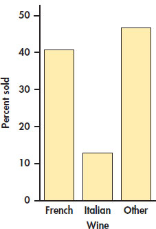
| Percent | 40.74 | 12.76 | 46.50 |
The total should be 100% because each bottle of wine sold is classified into exactly one of these three categories. In this case, the total is exactly 100%. Small deviations from 100% can occur due to roundoff error.
As usual, we prefer to display numerical summaries using a graph. Figure 2.21 is a bar graph of the distribution of wine type sold. In a two-way table, we have two marginal distributions, one for each of the variables that defines the table.
APPLY YOUR KNOWLEDGE
Question 1.91 Marginal distribution for type of music
CASE 2.2 Find the marginal distribution for the type of music. Display the distribution using a graph.
In working with two-way tables, you must calculate lots of percents. Here’s a tip to help you decide what fraction gives the percent you want. Ask, “What group represents the total that I want a percent of?” The count for that group is the denominator of the fraction that leads to the percent. In Example 2.25, we wanted percents “of bottles of the different types of wine sold,” so the table total is the denominator.
APPLY YOUR KNOWLEDGE
Question 1.92 Construct a two-way table
Construct your own 2 × 3 table. Add the marginal totals and find the two marginal distributions.
Question 1.93 Fields of study for college students

The following table gives the number of students (in thousands) graduating from college with degrees in several fields of study for seven countries:15
107
| Field of study | Canada | France | Germany | Italy | Japan | U.K. | U.S. |
|---|---|---|---|---|---|---|---|
| Social sciences, business, law | 64 | 153 | 66 | 125 | 259 | 152 | 878 |
| Science, mathematics, engineering | 35 | 111 | 66 | 80 | 136 | 128 | 355 |
| Arts and humanities | 27 | 74 | 33 | 42 | 123 | 105 | 397 |
| Education | 20 | 45 | 18 | 16 | 39 | 14 | 167 |
| Other | 30 | 289 | 35 | 58 | 97 | 76 | 272 |
- Calculate the marginal totals, and add them to the table.
- Find the marginal distribution of country, and give a graphical display of the distribution.
- Do the same for the marginal distribution of field of study.
Conditional distributions
The 3 × 3 table for Case 2.2 contains much more information than the two marginal distributions. We need to do a little more work to describe the relationship between the type of music playing and the type of wine purchased. Relationships among categorical variables are described by calculating appropriate percents from the counts given.
Conditional Distributions
To find the conditional distribution of the column variable for a particular value of the row variable in a two-way table, divide each count in the row by the row total. Similarly, to find the conditional distribution of the row variable for a particular value of the column variable in a two-way table, divide each count in the column by the column total.
EXAMPLE 2.26: Wine Purchased When No Music Was Playing
CASE 2.2 What types of wine were purchased when no music was playing? To answer this question, we find the marginal distribution of wine type for the value of music equal to none. The counts we need are in the first column of our table:
| Music | |
|---|---|
| Wine | None |
| French | 30 |
| Italian | 11 |
| Other | 43 |
| Total | 84 |
What percent of French wine was sold when no music was playing? To answer this question, we divide the number of bottles of French wine sold when no music was playing by the total number of bottles of wine sold when no music was playing:
108
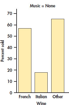
In the same way, we calculate the percents for Italian and other types of wine. Here are the results:
| Wine type: | French | Italian | Other |
| Percent when no music is playing: | 35.7 | 13.1 | 51.2 |
Other wine was the most popular choice when no music was playing, but French wine has a reasonably large share. Notice that these percents sum to 100%. There is no roundoff error here. The distribution is displayed in Figure 2.22.
APPLY YOUR KNOWLEDGE
Question 1.94 Conditional distribution when French music was playing
- Write down the column of counts that you need to compute the conditional distribution of the type of wine sold when French music was playing.
- Compute this conditional distribution.
- Display this distribution graphically.
- Compare this distribution with the one in Example 2.26. Was there an increase in sales of French wine when French music was playing rather than no music?
Question 1.95 Conditional distribution when Italian music was playing
- Write down the column of counts that you need to compute the conditional distribution of the type of wine sold when Italian music was playing.
- Compute this conditional distribution.
- Display this distribution graphically.
- Compare this distribution with the one in Example 2.26. Was there an increase in sales of Italian wine when Italian music was playing rather than no music?
Question 1.96 Compare the conditional distributions
In Example 2.26, we found the distribution of sales by wine type when no music was playing. In Exercise 2.94, you found the distribution when French music was playing, and in Exercise 2.95, you found the distribution when Italian music was playing. Examine these three conditional distributions carefully, and write a paragraph summarizing the relationship between sales of different types of wine and the music played.
109
For Case 2.2, we examined the relationship between sales of different types of wine and the music that was played by studying the three conditional distributions of type of wine sold, one for each music condition. For these computations, we used the counts from the 3 × 3 table, one column at a time. We could also have computed conditional distributions using the counts for each row. The result would be the three conditional distributions of the type of music played for each of the three wine types. For this example, we think that conditioning on the type of music played gives us the most useful data summary. Comparing conditional distributions can be particularly useful when the column variable is an explanatory variable.

The choice of which conditional distribution to use depends on the nature of the data and the questions that you want to ask. Sometimes you will prefer to condition on the column variable, and sometimes you will prefer to condition on the row variable. Occasionally, both sets of conditional distributions will be useful. Statistical software will calculate all of these quantities. You need to select the parts of the output that are needed for your particular questions. Don’t let computer software make this choice for you.
APPLY YOUR KNOWLEDGE
Question 1.97 Fields of study by country for college students
In Exercise 2.93, you examined data on fields of study for graduating college students from seven countries.
- Find the seven conditional distributions giving the distribution of graduates in the different fields of study for each country.
- Display the conditional distributions graphically.
- Write a paragraph summarizing the relationship between field of study and country.
Question 1.98 Countries by fields of study for college students
Refer to the previous exercise. Answer the same questions for the conditional distribution of country for each field of study.
Question 1.99 Compare the two analytical approaches
In the previous two exercises, you examined the relationship between country and field of study in two different ways.
- Compare these two approaches.
- Which do you prefer? Give a reason for your answer.
- What kinds of questions are most easily answered by each of the two approaches? Explain your answer.
Mosaic plots and software output
Statistical software will compute all of the quantities that we have discussed in this section. Included in some output is a very useful graphical summary called a mosaic plot. Here is an example.
mosaic plot
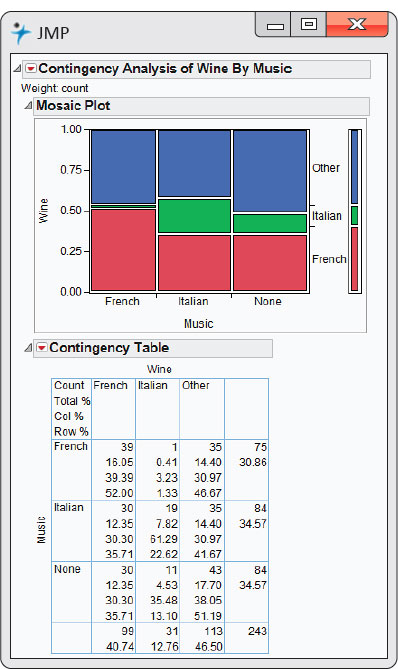
EXAMPLE 2.27: Software Output for Wine and Music
CASE 2.2 Output from JMP statistical software for the wine and music data is given in Figure 2.23. The mosaic plot is given in the top part of the display. Here, we think of music as the explanatory variable and wine as the response variable, so music is displayed across the x axis in the plot. The conditional distributions of wine for each type of music are displayed in the three columns. Note that when French is playing, 52% of the wine sold is French wine. The red bars display the percents of French wine sold for each type of music. Similarly, the green and blue bars display the correspondence to Italian wine and other wine, respectively. The widths of the three sets of bars display the marginal distribution of music. We can see that the proportions are approximately equal, but the French wine sold a little less than the other two categories of wine.
Simpson’s paradox
As is the case with quantitative variables, the effects of lurking variables can change or even reverse relationships between two categorical variables. Here is an example that demonstrates the surprises that can await the unsuspecting user of data.
EXAMPLE 2.28: Which Customer Service Representative Is Better?

A customer service center has a goal of resolving customer questions in 10 minutes or less. Here are the records for two representatives:
| Representative | ||
|---|---|---|
| Goal met | Ashley | Joshua |
| Yes | 172 | 118 |
| No | 28 | 82 |
| Total | 200 | 200 |
Ashley has met the goal 172 times out of 200, a success rate of 86%. For Joshua, the success rate is 118 out of 200, or 59%. Ashley clearly has the better success rate.
111
Let’s look at the data in a little more detail. The data summarized come from two different weeks in the year.
EXAMPLE 2.29: Let’s Look at the Data More Carefully
Here are the counts broken down by week:
| Week 1 | Week 2 | |||
|---|---|---|---|---|
| Goal met | Ashley | Joshua | Ashley | Joshua |
| Yes | 162 | 19 | 10 | 99 |
| No | 18 | 1 | 10 | 81 |
| Total | 180 | 20 | 20 | 180 |
For Week 1, Ashley met the goal 90% of the time (162/180), while Joshua met the goal 95% of the time (19/20). Joshua had the better performance in Week 1. What about Week 2? Here, Ashley met the goal 50% of the time (10/20), while the success rate for Joshua was 55% (99/180). Joshua again had the better performance. How does this analysis compare with the analysis that combined the counts for the two weeks? That analysis clearly showed that Ashley had the better performance, 86% versus 59%.
These results can be explained by a lurking variable related to week. The first week was during a period when the product had been in use for several months. Most of the calls to the customer service center concerned problems that had been encountered before. The representatives were trained to answer these questions and usually had no trouble in meeting the goal of resolving the problems quickly. On the other hand, the second week occurred shortly after the release of a new version of the product. Most of the calls during this week concerned new problems that the representatives had not yet encountered. Many more of these questions took longer than the 10-minute goal to resolve.
Look at the total in the bottom row of the detailed table. During the first week, when calls were easy to resolve, Ashley handled 180 calls and Joshua handled 20. The situation was exactly the opposite during the second week, when calls were difficult to resolve. There were 20 calls for Ashley and 180 for Joshua.
The original two-way table, which did not take account of week, was misleading. This example illustrates Simpson’s paradox.
Simpson’s Paradox
An association or comparison that holds for all of several groups can reverse direction when the data are combined to form a single group. This reversal is called Simpson’s paradox.
The lurking variables in Simpson’s paradox are categorical. That is, they break the cases into groups, as when calls are classified by week. Simpson’s paradox is just an extreme form of the fact that observed associations can be misleading when there are lurking variables.
APPLY YOUR KNOWLEDGE
Question 1.100 Which hospital is safer?

Insurance companies and consumers are interested in the performance of hospitals. The government releases data about patient outcomes in hospitals that can be useful in making informed health care decisions. Here is a two-way table of data on the survival of patients after surgery in two hospitals. All patients undergoing surgery in a recent time period are included. “Survived” means that the patient lived at least six weeks following surgery.
112
| Hospital A | Hospital B | |
|---|---|---|
| Died | 63 | 16 |
| Survived | 2037 | 784 |
| Total | 2100 | 800 |
What percent of Hospital A patients died? What percent of Hospital B patients died? These are the numbers one might see reported in the media.
Question 1.101 Patients in “poor” or “good” condition
Not all surgery cases are equally serious, however. Patients are classified as being in either “poor” or “good” condition before surgery. Here are the data broken down by patient condition. Check that the entries in the original two-way table are just the sums of the “poor” and “good” entries in this pair of tables.
| Good Condition | ||
|---|---|---|
| Hospital A | Hospital B | |
| Died | 6 | 8 |
| Survived | 594 | 592 |
| Total | 600 | 600 |
| Poor Condition | ||
| Hospital A | Hospital B | |
|---|---|---|
| Died | 57 | 8 |
| Survived | 1443 | 192 |
| Total | 1500 | 200 |
- Find the percent of Hospital A patients who died who were classified as “poor” before surgery. Do the same for Hospital B. In which hospital do “poor” patients fare better?
- Repeat part (a) for patients classified as “good” before surgery.
- What is your recommendation to someone facing surgery and choosing between these two hospitals?
- How can Hospital A do better in both groups, yet do worse overall? Look at the data and carefully explain how this can happen.
The data in Example 2.28 can be given in a three-way table that reports counts for each combination of three categorical variables: week, representative, and whether or not the goal was met. In Example 2.29, we constructed two two-way tables for representative by goal, one for each week. The original table, the one that we showed in Example 2.28, can be obtained by adding the corresponding counts for the two tables in Example 2.29. This process is called aggregating the data. When we aggregated data in Example 2.28, we ignored the variable week, which then became a lurking variable. Conclusions that seem obvious when we look only at aggregated data can become quite different when the data are examined in more detail.
three-way table
aggregation
SECTION 2.5 Summary
- A two-way table of counts organizes counts of data classified by two categorical variables. Values of the row variable label the rows that run across the table, and values of the column variable label the columns that run down the table. Two-way tables are often used to summarize large amounts of information by grouping outcomes into categories.
- The row totals and column totals in a two-way table give the marginal distributions of the two individual variables. It is clearer to present these distributions as percents of the table total. Marginal distributions tell us nothing about the relationship between the variables.
- To find the conditional distribution of the row variable for one specific value of the column variable, look only at that one column in the table. Divide each entry in the column by the column total.
- There is a conditional distribution of the row variable for each column in the table. Comparing these conditional distributions is one way to describe the association between the row and the column variables. It is particularly useful when the column variable is the explanatory variable.
- Bar graphs are a flexible means of presenting categorical data. There is no single best way to describe an association between two categorical variables.
- Mosaic plots are effective graphical displays for two-way tables, particularly when the column variable is an explanatory variable.
- A comparison between two variables that holds for each individual value of a third variable can be changed or even reversed when the data for all values of the third variable are combined. This is Simpson’s paradox. Simpson’s paradox is an example of the effect of lurking variables on an observed association.
SECTION 2.5 Exercises
For Exercise 2.91, see page 106; for 2.92 and 2.93, see pages 106–107; for 2.94 to 2.96, see page 108; for 2.97 to 2.99, see page 109; and for 2.100 and 2.101, see pages 111–112.
Question 1.102 Remote deposit capture
The Federal Reserve has called remote deposit capture (RDC) “the most important development the [U.S.] banking industry has seen in years.” This service allows users to scan checks and to transmit the scanned images to a bank for posting.16 In its annual survey of community banks, the American Bankers Association asked banks whether or not they offered this service.17 Here are the results classified by the asset size (in millions of dollars) of the bank: 
| Offer RDC | ||
|---|---|---|
| Asset size ($ in millions) |
Yes | No |
| Under $100 | 63 | 309 |
| $101 to $200 | 59 | 132 |
| $201 or more | 112 | s85 |
Summarize the results of this survey question numerically and graphically. Write a short paragraph explaining the relationship between the size of a bank, measured by assets, and whether or not RDC is offered.
Question 1.103 How does RDC vary across the country?
The survey described in the previous exercise also classified community banks by region. Here is the 6 × 2 table of counts:18 
| Offer RDC | ||
|---|---|---|
| Region | Yes | No |
| Northeast | 28 | 38 |
| Southeast | 57 | 61 |
| Central | 53 | 84 |
| Midwest | 63 | 181 |
| Southwest | 27 | 51 |
| West | 61 | 76 |
Summarize the results of this survey question numerically and graphically. Write a short paragraph explaining the relationship between the location of a bank, measured by region, and whether or not remote deposit capture is offered.
Question 1.104 Exercise and adequate sleep
A survey of 656 boys and girls, ages 13 to 18, asked about adequate sleep and other health-related behaviors. The recommended amount of sleep is six to eight hours per night.19 In the survey, 54% of the respondents reported that they got less than this amount of sleep on school nights. The researchers also developed an exercise scale that was used to classify the students as above or below the median in how much they exercised. Here is the 2 × 2 table of counts with students classified as getting or not getting adequate sleep and by the exercise variable: 
114
| Exercise | ||
|---|---|---|
| Enough sleep | High | Low |
| Yes | 151 | 115 |
| No | 148 | 242 |
- Find the distribution of adequate sleep for the high exercisers.
- Do the same for the low exercisers.
- If you have the appropriate software, use a mosaic plot to illustrate the marginal distribution of exercise and your results in parts (a) and (b).
- Summarize the relationship between adequate sleep and exercise using the results of parts (a) and (b).
Question 1.105 Adequate sleep and exercise
Refer to the previous exercise.
- Find the distribution of exercise for those who get adequate sleep.
- Do the same for those who do not get adequate sleep.
- Write a short summary of the relationship between adequate sleep and exercise using the results of parts (a) and (b).
- Compare this summary with the summary that you obtained in part (c) of the previous exercise. Which do you prefer? Give a reason for your answer.
Question 1.106 Full-time and part-time college students
The Census Bureau provides estimates of numbers of people in the United States classified in various ways.20 Let’s look at college students. The following table gives us data to examine the relation between age and full-time or part-time status. The numbers in the table are expressed as thousands of U.S. college students. 
| Status | ||
|---|---|---|
| Age | Full-time | Part-time |
| 15–19 | 3388 | 389 |
| 20–24 | 5238 | 1164 |
| 25–34 | 1703 | 1699 |
| 35 and over | 762 | 2045 |
- Find the distribution of age for full-time students.
- Do the same for the part-time students.
- Use the summaries in parts (a) and (b) to describe the relationship between full- or part-time status and age. Write a brief summary of your conclusions.
Question 1.107 Condition on age
Refer to the previous exercise.
- For each age group, compute the percent of students who are full-time and the percent of students who are part-time.
- Make a graphical display of the results that you found in part (a).
- If you have the appropriate software, make a mosaic plot.
- In a short paragraph, describe the relationship between age and full- or part-time status using your numerical and graphical summaries.
- Explain why you need only the percents of students who are full-time for your summary in part (b).
- Compare this way of summarizing the relationship between these two variables with what you presented in part (c) of the previous exercise.
Question 1.108 Lying to a teacher
One of the questions in a survey of high school students asked about lying to teachers.21 The accompanying table gives the numbers of students who said that they lied to a teacher about something significant at least once during the past year, classified by gender. 
| Gender | ||
|---|---|---|
| Lied at least once | Male | Female |
| Yes | 6067 | 5966 |
| No | 4145 | 5719 |
- Add the marginal totals to the table.
- Calculate appropriate percents to describe the results of this question.
- Summarize your findings in a short paragraph.
Question 1.109 Trust and honesty in the workplace
The students surveyed in the study described in the previous exercise were also asked whether they thought trust and honesty were essential in business and the workplace. Here are the counts classified by gender: 
| Gender | ||
|---|---|---|
| Trust and honesty are essential | Male | Female |
| Agree | 9,097 | 10,935 |
| Disagree | 685 | 423 |
Answer the questions given in the previous exercise for this survey question.
115
Question 1.110 Class size and course level
College courses taught at lower levels often have larger class sizes. The following table gives the number of classes classified by course level and class size.22 For example, there were 202 first-year level courses with between one and nine students. 
| Class size | |||||||
|---|---|---|---|---|---|---|---|
| Course level |
1–9 | 10–19 | 20–29 | 30–39 | 40–49 | 50–99 | 100 or more |
| 1 | 202 | 659 | 917 | 241 | 70 | 99 | 123 |
| 2 | 190 | 370 | 486 | 307 | 84 | 109 | 134 |
| 3 | 150 | 387 | 314 | 115 | 96 | 186 | 53 |
| 4 | 146 | 256 | 190 | 83 | 67 | 64 | 17 |
- Fill in the marginal totals in the table.
- Find the marginal distribution for the variable course level.
- Do the same for the variable class size.
- For each course level, find the conditional distribution of class size.
- Summarize your findings in a short paragraph.
Question 1.111 Hiring practices
A company has been accused of age discrimination in hiring for operator positions. Lawyers for both sides look at data on applicants for the past three years. They compare hiring rates for applicants younger than 40 years and those 40 years or older. 
| Age | Hired | Not hired |
|---|---|---|
| Younger than 40 | 82 | 1160 |
| 40 or older | 2 | 168 |
- Find the two conditional distributions of hired/not hired—one for applicants who are less than 40 years old and one for applicants who are not less than 40 years old.
- Based on your calculations, make a graph to show the differences in distribution for the two age categories.
- Describe the company’s hiring record in words. Does the company appear to discriminate on the basis of age?
- What lurking variables might be involved here?
Question 1.112 Nonresponse in a survey of companies
A business school conducted a survey of companies in its state. It mailed a questionnaire to 200 small companies, 200 medium-sized companies, and 200 large companies. The rate of nonresponse is important in deciding how reliable survey results are. Here are the data on response to this survey: 
| Small | Medium | Large | |
|---|---|---|---|
| Response | 124 | 80 | 41 |
| No response | 76 | 120 | 159 |
| Total | 200 | 200 | 200 |
- What was the overall percent of nonresponse?
- Describe how nonresponse is related to the size of the business. (Use percents to make your statements precise.)
- Draw a bar graph to compare the nonresponse percents for the three size categories.
Question 1.113 Demographics and new products
Companies planning to introduce a new product to the market must define the “target” for the product. Who do we hope to attract with our new product? Age and gender are two of the most important demographic variables. The following two-way table describes the age and marital status of American women.23 The table entries are in thousands of women. 
| Marital status | ||||
|---|---|---|---|---|
| Age (years) | Never married |
Married | Widowed | Divorced |
| 18 to 24 | 12,112 | 2,171 | 23 | 164 |
| 25 to 39 | 9,472 | 18,219 | 177 | 2,499 |
| 40 to 64 | 5,224 | 35,021 | 2,463 | 8,674 |
| ≥ 65 | 984 | 9,688 | 8,699 | 2,412 |
- Find the sum of the entries for each column.
- Find the marginal distributions.
- Find the conditional distributions.
- If you have the appropriate software, make a mosaic plot.
- Write a short description of the relationship between marital status and age for women.
Question 1.114 Demographics, continued
- Using the data in the previous exercise, compare the conditional distributions of marital status for women aged 18 to 24 and women aged 40 to 64. Briefly describe the most important differences between the two groups of women, and back up your description with percents.
- Your company is planning a magazine aimed at women who have never been married. Find the conditional distribution of age among never-married women, and display it in a bar graph. What age group or groups should your magazine aim to attract?
Question 1.115 Demographics and new products—men
Refer to Exercises 2.113 and 2.114. Here are the corresponding counts for men:
116
| Marital status | ||||
|---|---|---|---|---|
| Age (years) | Never married |
Married | Widowed | Divorced |
| 18 to 24 | 13,509 | 1,245 | 6 | 63 |
| 25 to 39 | 12,685 | 16,029 | 78 | 1,790 |
| 40 to 64 | 6,869 | 34,650 | 760 | 6,647 |
| ≥ 65 | 685 | 12,514 | 2,124 | 1,464 |
Answer the questions from Exercises 2.113 and 2.114 for these counts.
Question 1.116 Discrimination?
Wabash Tech has two professional schools, business and law. Here are two-way tables of applicants to both schools, categorized by gender and admission decision. (Although these data are made up, similar situations occur in reality.) 
| Business | ||
|---|---|---|
| Admit | Deny | |
| Male | 480 | 120 |
| Female | 180 | 20 |
| Law | ||
|---|---|---|
| Admit | Deny | |
| Male | 10 | 90 |
| Female | 100 | 200 |
- Make a two-way table of gender by admission decision for the two professional schools together by summing entries in these tables.
- From the two-way table, calculate the percent of male applicants who are admitted and the percent of female applicants who are admitted. Wabash admits a higher percent of male applicants.
- Now compute separately the percents of male and female applicants admitted by the business school and by the law school. Each school admits a higher percent of female applicants.
- This is Simpson’s paradox: both schools admit a higher percent of the women who apply, but overall, Wabash admits a lower percent of female applicants than of male applicants. Explain carefully, as if speaking to a skeptical reporter, how it can happen that Wabash appears to favor males when each school individually favors females.
Question 1.117 Obesity and health
Recent studies have shown that earlier reports underestimated the health risks associated with being overweight. The error was due to lurking variables. In particular, smoking tends both to reduce weight and to lead to earlier death. Illustrate Simpson’s paradox by a simplified version of this situation. That is, make up tables of overweight (yes or no) by early death (yes or no) by smoker (yes or no) such that
- Overweight smokers and overweight nonsmokers both tend to die earlier than those not overweight.
- But when smokers and nonsmokers are combined into a two-way table of overweight by early death, persons who are not overweight tend to die earlier.
Question 1.118 Find the table
Here are the row and column totals for a two-way table with two rows and two columns:
| a | b | 60 |
| c | d | 60 |
| 70 | 50 | 120 |
Find two different sets of counts a, b, c, and d for the body of the table that give these same totals. This shows that the relationship between two variables cannot be obtained from the two individual distributions of the variables.
CHAPTER 2 Review Exercises
Question 1.119 Companies of the world with logs
In Exercises 2.10 (page 72), 2.27 (page 78), and 2.58 (pages 95–96), you examined the relationship between the numbers of companies that are incorporated and are listed on their country’s stock exchange at the end of the year using data collected by the World Bank.24 In this exercise, you will explore the relationship between the numbers for 2012 and 2002 using logs.

- Which variable do you choose to be the explanatory variable, and which do you choose to be the response variable? Explain your answer.
- Plot the data with the least-squares regression line. Summarize the major features of your plot.
- Give the equation of the least-squares regression line.
- Find the predicted value and the residual for Sweden.
- Find the correlation between the two variables.
- Compare the results found in this exercise with those you found in Exercises 2.10, 2.27, and 2.58. Do you prefer the analysis with the original data or the analysis using logs? Give reasons for your answer.
117
Question 1.120 Residuals for companies of the world with logs
Refer to the previous exercise.
- Use a histogram to examine the distribution of the residuals.
- Make a Normal quantile plot of the residuals.
- Summarize the distribution of the residuals using the graphical displays that you created in parts (a) and (b).
- Repeat parts (a), (b), and (c) for the original data, and compare these results with those you found in parts (a), (b), and (c). Which do you prefer? Give reasons for your answer.
Question 1.121 Dwelling permits and sales for 21 European countries
The Organization for Economic Cooperation and Development (OECD) collects data on Main Economic Indicators (MEIs) for many countries. Each variable is recorded as an index, with the year 2000 serving as a base year. This means that the variable for each year is reported as a ratio of the value for the year divided by the value for 2000. Use of indices in this way makes it easier to compare values for different countries.25 
- Make a scatterplot with sales as the response variable and permits issued for new dwellings as the explanatory variable. Describe the relationship. Are there any outliers or influential observations?
- Find the least-squares regression line and add it to your plot.
- What is the predicted value of sales for a country that has an index of 160 for dwelling permits?
- The Netherlands has an index of 160 for dwelling permits. Find the residual for this country.
- What percent of the variation in sales is explained by dwelling permits?
Question 1.122 Dwelling permits and production
Refer to the previous exercise.
- Make a scatterplot with production as the response variable and permits issued for new dwellings as the explanatory variable. Describe the relationship. Are there any outliers or influential observations?
- Find the least-squares regression line and add it to your plot.
- What is the predicted value of production for a country that has an index of 160 for dwelling permits?
- The Netherlands has an index of 160 for dwelling permits. Find the residual for this country.
- What percent of the variation in production is explained by dwelling permits? How does this value compare with the value you found in the previous exercise for the percent of variation in sales that is explained by building permits?
Question 1.123 Sales and production
Refer to the previous two exercises.
- Make a scatterplot with sales as the response variable and production as the explanatory variable. Describe the relationship. Are there any outliers or influential observations?
- Find the least-squares regression line and add it to your plot.
- What is the predicted value of sales for a country that has an index of 125 for production?
- Finland has an index of 125 for production. Find the residual for this country.
- What percent of the variation in sales is explained by production? How does this value compare with the percents of variation that you calculated in the two previous exercises?
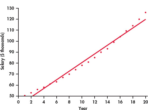
Question 1.124 Salaries and raises
For this exercise, we consider a hypothetical employee who starts working in Year 1 at a salary of $50,000. Each year her salary increases by approximately 5%. By Year 20, she is earning $126,000. The following table gives her salary for each year (in thousands of dollars): 
| Year | Salary | Year | Salary | Year | Salary | Year | Salary |
|---|---|---|---|---|---|---|---|
| 1 | 50 | 6 | 63 | 11 | 81 | 16 | 104 |
| 2 | 53 | 7 | 67 | 12 | 85 | 17 | 109 |
| 3 | 56 | 8 | 70 | 13 | 90 | 18 | 114 |
| 4 | 58 | 9 | 74 | 14 | 93 | 19 | 120 |
| 5 | 61 | 10 | 78 | 15 | 99 | 20 | 126 |
- Figure 2.24 is a scatterplot of salary versus year with the least-squares regression line. Describe the relationship between salary and year for this person.
- The value of r2 for these data is 0.9832. What percent of the variation in salary is explained by year? Would you say that this is an indication of a strong linear relationship? Explain your answer.
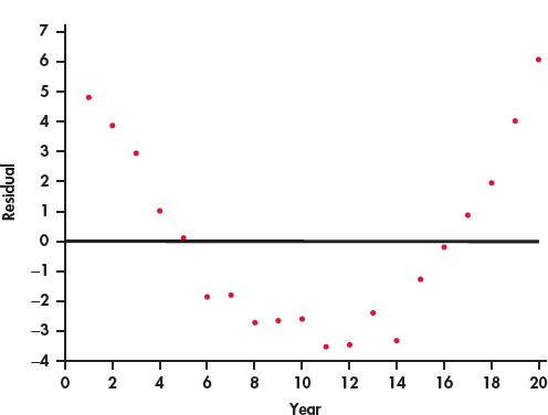
Question 1.125 Look at the residuals
Refer to the previous exercise. Figure 2.25 is a plot of the residuals versus year.
- Interpret the residual plot.
- Explain how this plot highlights the deviations from the least-squares regression line that you can see in Figure 2.24.
118
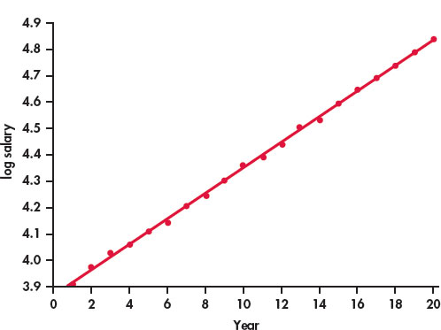
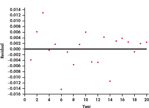
Question 1.126 Try logs
Refer to the previous two exercises. Figure 2.26 is a scatterplot with the least-squares regression line for log salary versus year. For this model, r2 = 0.9995.
- Compare this plot with Figure 2.24. Write a short summary of the similarities and the differences.
- Figure 2.27 is a plot of the residuals for the model using year to predict log salary. Compare this plot with Figure 2.25 and summarize your findings.
Question 1.127 Predict some salaries
The individual whose salary we have been studying in Exercises 2.122 through 2.124 wants to do some financial planning. Specifically, she would like to predict her salary five years into the future, that is, for Year 25. She is willing to assume that her employment situation will be stable for the next five years and that it will be similar to the last 20 years.
- Use the least-squares regression equation constructed to predict salary from year to predict her salary for Year 25.
- Use the least-squares regression equation constructed to predict log salary from year to predict her salary for Year 25. Note that you will need to convert the predicted log salary back to the predicted salary. Many calculators have a function that will perform this operation.
- Which prediction do you prefer? Explain your answer.
- Someone looking at the numerical summaries, and not the plots, for these analyses says that because both models have very high values of r2, they should perform equally well in doing this prediction. Write a response to this comment.
- Write a short paragraph about the value of graphical summaries and the problems of extrapolation using what you have learned from studying these salary data.
119
Question 1.128 Faculty salaries
Data on the salaries of a sample of professors in a business department at a large university are given below. The salaries are for the academic years 2014–2015 and 2015–2016. 
| 2014–2015 salary ($) |
2015–2016 salary ($) |
2014–2015 salary ($) |
2015–2016 salary ($) |
|---|---|---|---|
| 145,700 | 147,700 | 136,650 | 138,650 |
| 112,700 | 114,660 | 132,160 | 134,150 |
| 109,200 | 111,400 | 74,290 | 76,590 |
| 98,800 | 101,900 | 74,500 | 77,000 |
| 112,000 | 113,000 | 83,000 | 85,400 |
| 111,790 | 113,800 | 141,850 | 143,830 |
| 103,500 | 105,700 | 122,500 | 124,510 |
| 149,000 | 150,900 | 115,100 | 117,100 |
- Construct a scatterplot with the 2015–2016 salaries on the vertical axis and the 2014–2015 salaries on the horizontal axis.
- Comment on the form, direction, and strength of the relationship in your scatterplot.
- What proportion of the variation in 2015–2016 salaries is explained by 2014–2015 salaries?
Question 1.129 Find the line and examine the residuals
Refer to the previous exercise.
- Find the least-squares regression line for predicting 2015–2016 salaries from 2014–2015 salaries.
- Analyze the residuals, paying attention to any outliers or influential observations. Write a summary of your findings.
Question 1.130 Bigger raises for those earning less
Refer to the previous two exercises. The 2014–2015 salaries do an excellent job of predicting the 2015–2016 salaries. Is there anything more that we can learn from these data? In this department, there is a tradition of giving higher-than-average percent raises to those whose salaries are lower. Let’s see if we can find evidence to support this idea in the data.
120
- Compute the percent raise for each faculty member. Take the difference between the 2015–2016 salary and the 2014–2015 salary, divide by the 2014–2015 salary, and then multiply by 100. Make a scatterplot with the raise as the response variable and the 2014–2015 salary as the explanatory variable. Describe the relationship that you see in your plot.
- Find the least-squares regression line and add it to your plot.
- Analyze the residuals. Are there any outliers or influential cases? Make a graphical display and include it in a short summary of what you conclude.
- Is there evidence in the data to support the idea that greater percentage raises are given to those with lower salaries? Summarize your findings and include numerical and graphical summaries to support your conclusion.
Question 1.131 Marketing your college
Colleges compete for students, and many students do careful research when choosing a college. One source of information is the rankings compiled by U.S. News & World Report. One of the factors used to evaluate undergraduate programs is the proportion of incoming students who graduate. This quantity, called the graduation rate, can be predicted by other variables such as the SAT or ACT scores and the high school records of the incoming students. One of the components in U.S. News & World Report rankings is the difference between the actual graduation rate and the rate predicted by a regression equation.26 In this chapter, we call this quantity the residual. Explain why the residual is a better measure to evaluate college graduation rates than the raw graduation rate.
Question 1.132 Planning for a new product
The editor of a statistics text would like to plan for the next edition. A key variable is the number of pages that will be in the final version. Text files are prepared by the authors using a word processor called LaTeX, and separate files contain figures and tables. For the previous edition of the text, the number of pages in the LaTeX files can easily be determined, as well as the number of pages in the final version of the text. Here are the data: 
| Chapter | |||||||||||||
|---|---|---|---|---|---|---|---|---|---|---|---|---|---|
| 1 | 2 | 3 | 4 | 5 | 6 | 7 | 8 | 9 | 10 | 11 | 12 | 13 | |
| LaTeX pages |
77 | 73 | 59 | 80 | 45 | 66 | 81 | 45 | 47 | 43 | 31 | 46 | 26 |
| Text pages |
99 | 89 | 61 | 82 | 47 | 68 | 87 | 45 | 53 | 50 | 36 | 52 | 19 |
- Plot the data and describe the overall pattern.
- Find the equation of the least-squares regression line, and add the line to your plot.
- Find the predicted number of pages for the next edition if the number of LaTeX pages for a chapter is 62.
- Write a short report for the editor explaining to her how you constructed the regression equation and how she could use it to estimate the number of pages in the next edition of the text.
Question 1.133 Points scored in women’s basketball games
Use the Internet to find the scores for the past season’s women’s basketball team at a college of your choice. Is there a relationship between the points scored by your chosen team and the points scored by their opponents? Summarize the data and write a report on your findings.
Question 1.134 Look at the data for men
Refer to the previous exercise. Analyze the data for the men’s team from the same college, and compare your results with those for the women.
Question 1.135 Circular saws
The following table gives the weight (in pounds) and amps for 19 circular saws. Saws with higher amp ratings tend to also be heavier than saws with lower amp ratings. We can quantify this fact using regression. 
| Weight | Amps | Weight | Amps | Weight | Amps |
|---|---|---|---|---|---|
| 11 | 15 | 9 | 10 | 11 | 13 |
| 12 | 15 | 11 | 15 | 13 | 14 |
| 11 | 15 | 12 | 15 | 10 | 12 |
| 11 | 15 | 12 | 14 | 11 | 12 |
| 12 | 15 | 10 | 10 | 11 | 12 |
| 11 | 15 | 12 | 13 | 10 | 12 |
| 13 | 15 |
- We will use amps as the explanatory variable and weight as the response variable. Give a reason for this choice.
- Make a scatterplot of the data. What do you notice about the weight and amp values?
- Report the equation of the least-squares regression line along with the value of r2.
- Interpret the value of the estimated slope.
- How much of an increase in amps would you expect to correspond to a one-pound increase in the weight of a saw, on average, when comparing two saws?
- Create a residual plot for the model in part (b). Does the model indicate curvature in the data?
121
Question 1.136 Circular saws
The table in the previous exercise gives the weight (in pounds) and amps for 19 circular saws. The data contain only five different amp ratings among the 19 saws.
- Calculate the correlation between the weights and the amps of the 19 saws.
- Calculate the average weight of the saws for each of the five amp ratings.
- Calculate the correlation between the average weights and the amps. Is the correlation between average weights and amps greater than, less than, or equal to the correlation between individual weights and amps?
Question 1.137 What correlation does and doesn’t say
Construct a set of data with two variables that have different means and correlation equal to one. Use your example to illustrate what correlation does and doesn’t say.
Question 1.138 Simpson’s paradox and regression
Simpson’s paradox occurs when a relationship between variables within groups of observations reverses when all of the data are combined. The phenomenon is usually discussed in terms of categorical variables, but it also occurs in other settings. Here is an example: 
| y | x | Group | y | x | Group |
|---|---|---|---|---|---|
| 10.1 | 1 | 1 | 18.3 | 6 | 2 |
| 8.9 | 2 | 1 | 17.1 | 7 | 2 |
| 8.0 | 3 | 1 | 16.2 | 8 | 2 |
| 6.9 | 4 | 1 | 15.1 | 9 | 2 |
| 6.1 | 5 | 1 | 14.3 | 10 | 2 |
- Make a scatterplot of the data for Group 1. Find the least-squares regression line and add it to your plot. Describe the relationship between y and x for Group 1.
- Do the same for Group 2.
- Make a scatterplot using all 10 observations. Find the least-squares line and add it to your plot.
- Make a plot with all of the data using different symbols for the two groups. Include the three regression lines on the plot. Write a paragraph about Simpson’s paradox for regression using this graphical display to illustrate your description.
Question 1.139 Wood products
A wood product manufacturer is interested in replacing solid-wood building material by less-expensive products made from wood flakes.27 The company collected the following data to examine the relationship between the length (in inches) and the strength (in pounds per square inch) of beams made from wood flakes: 
| Length | 5 | 6 | 7 | 8 | 9 | 10 | 11 | 12 | 13 | 14 |
| Strength | 446 | 371 | 334 | 296 | 249 | 254 | 244 | 246 | 239 | 234 |
- Make a scatterplot that shows how the length of a beam affects its strength.
- Describe the overall pattern of the plot. Are there any outliers?
- Fit a least-squares line to the entire set of data. Graph the line on your scatterplot. Does a straight line adequately describe these data?
- The scatterplot suggests that the relation between length and strength can be described by two straight lines, one for lengths of 5 to 9 inches and another for lengths of 9 to 14 inches. Fit least-squares lines to these two subsets of the data, and draw the lines on your plot. Do they describe the data adequately? What question would you now ask the wood experts?
Question 1.140 Aspirin and heart attacks
Does taking aspirin regularly help prevent heart attacks? “Nearly five decades of research now link aspirin to the prevention of stroke and heart attacks.” So says the Bayer Aspirin website, bayeraspirin.com. The most important evidence for this claim comes from the Physicians’ Health Study. The subjects were 22,071 healthy male doctors at least 40 years old. Half the subjects, chosen at random, took aspirin every other day. The other half took a placebo, a dummy pill that looked and tasted like aspirin. Here are the results.28 (The row for “None of these” is left out of the two-way table.)
| Aspirin group |
Placebo group |
|
|---|---|---|
| Fatal heart attacks | 10 | 26 |
| Other heart attacks | 129 | 213 |
| Strokes | 119 | 98 |
| Total | 11,037 | 11,034 |
What do the data show about the association between taking aspirin and heart attacks and stroke? Use percents to make your statements precise. Include a mosaic plot if you have access to the needed software. Do you think the study provides evidence that aspirin actually reduces heart attacks (cause and effect)? 
122
Question 1.141 More smokers live at least 20 more years!
You can see the headlines “More smokers than nonsmokers live at least 20 more years after being contacted for study!” A medical study contacted randomly chosen people in a district in England. Here are data on the 1314 women contacted who were either current smokers or who had never smoked. The tables classify these women by their smoking status and age at the time of the survey and whether they were still alive 20 years later.29 
| Age 18 to 44 | Age 45 to 64 | Age 65+ | ||||
|---|---|---|---|---|---|---|
| Smoker | Not | Smoker | Not | Smoker | Not | |
| Dead | 19 | 13 | 78 | 52 | 42 | 165 |
| Alive | 269 | 327 | 167 | 147 | 7 | 28 |
- From these data, make a two-way table of smoking (yes or no) by dead or alive. What percent of the smokers stayed alive for 20 years? What percent of the nonsmokers survived? It seems surprising that a higher percent of smokers stayed alive.
- The age of the women at the time of the study is a lurking variable. Show that within each of the three age groups in the data, a higher percent of nonsmokers remained alive 20 years later. This is another example of Simpson’s paradox.
- The study authors give this explanation: “Few of the older women (over 65 at the original survey) were smokers, but many of them had died by the time of follow-up.” Compare the percent of smokers in the three age groups to verify the explanation.
Question 1.142 Recycled product quality
Recycling is supposed to save resources. Some people think recycled products are lower in quality than other products, a fact that makes recycling less practical. People who actually use a recycled product may have different opinions from those who don’t use it. Here are data on attitudes toward coffee filters made of recycled paper among people who do and don’t buy these filters:30 
| Think the quality of the recycled product is: |
|||
|---|---|---|---|
| Higher | The same | Lower | |
| Buyers | 20 | 7 | 9 |
| Nonbuyers | 29 | 25 | 43 |
- Find the marginal distribution of opinion about quality. Assuming that these people represent all users of coffee filters, what does this distribution tell us?
- How do the opinions of buyers and nonbuyers differ? Use conditional distributions as a basis for your answer. Include a mosaic plot if you have access to the needed software. Can you conclude that using recycled filters causes more favorable opinions? If so, giving away samples might increase sales.