Should you splurge on a restaurant meal or save money by eating at home? Should you buy a new car and, if so, how expensive a model? Should you redo that bathroom or live with it for another year? In the real world, households are constantly confronted with such choices—not just about the consumption mix but also about how much to spend in total. These choices, in turn, have a powerful effect on the economy: consumer spending normally accounts for two-thirds of total spending on final goods and services. But what determines how much consumers spend?

The most important factor affecting a family’s consumer spending is its current disposable income—income after taxes are paid and government transfers are received. It’s obvious from daily life that people with high disposable incomes on average drive more expensive cars, live in more expensive houses, and spend more on meals and clothing than people with lower disposable incomes. And the relationship between current disposable income and spending is clear in the data.

163

The Bureau of Labor Statistics (BLS) collects annual data on family income and spending. Families are grouped by levels of before-tax income; after-tax income for each group is also reported. Since the income figures include transfers from the government, what the BLS calls a household’s after-tax income is equivalent to its current disposable income.

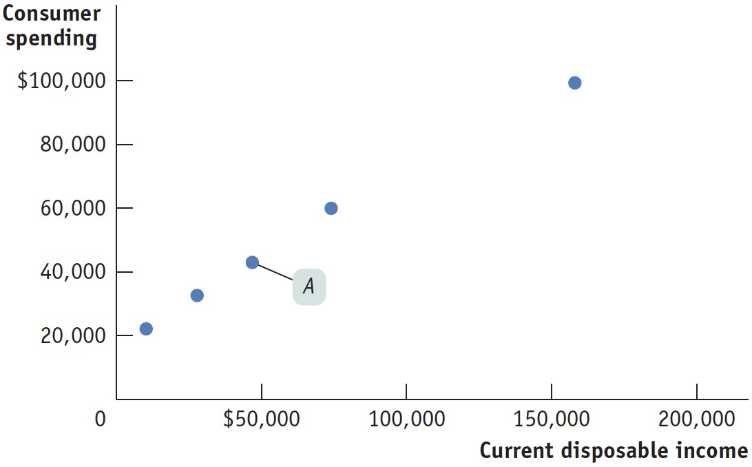
Figure 16.1 is a scatter diagram that illustrates the relationship between household current disposable income and household consumer spending for U.S. households by income group in 2012. For example, point A shows that in 2012 the middle fifth of the population had an average current disposable income of $46,777 and average spending of $43,004. The pattern of the dots slopes upward from left to right, making it clear that households with higher current disposable income had higher consumer spending.

A consumption function uses an equation or a graph to show how a household’s consumer spending varies with the household’s current disposable income.

Figure 16.2 provides the graph of a consumption function. The vertical intercept is the household’s autonomous consumer spending: the amount the household would spend if its current disposable income were zero. Autonomous consumer spending is greater than zero because a household with no disposable income can buy some things by borrowing or using its savings.

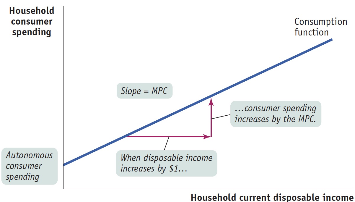
Recall that the marginal propensity to consume, or MPC, is the amount the household spends out of each additional $1 of current disposable income. The slope of any line is “rise over run”; for the consumption function, the rise is the increase in consumer spending and the run is the increase in current disposable income. For each $1 “run” in income, the “rise” is the MPC, so the slope of the consumption function is MPC/1 = MPC.

According to the data on U.S. households in Figure 16.1, the best estimate of autonomous consumption for that population in 2012 was $18,478 and the best estimate of MPC was $0.52. This implies that the marginal propensity to save (MPS)—the amount of an additional $1 of disposable income that is saved—is approximately 1 − 0.52 = 0.48 and the spending multiplier is 1/(1 − MPC) = 1/MPS = approximately 1/0.48 = 2.08.

An individual household’s consumption function shows a microeconomic relationship between the household’s current disposable income and its spending on goods and services. Macroeconomists study the aggregate consumption function, which shows the relationship between current disposable income and consumer spending for the economy as a whole. We can represent this relationship with the following equation:

164

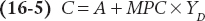
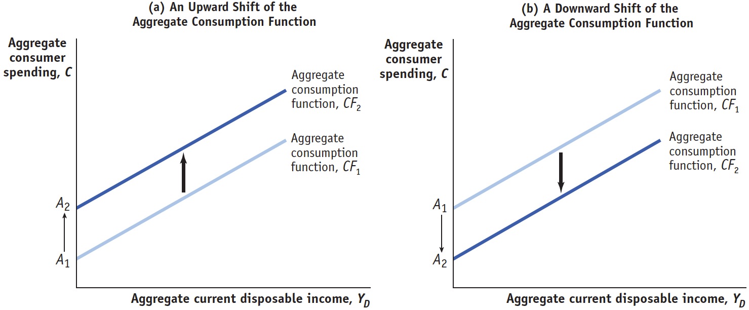
Here, C is aggregate consumer spending, Y_D is aggregate current disposable income, and A is aggregate autonomous consumer spending, the amount of consumer spending when disposable income is zero. Figure 16.3 shows two aggregate consumption functions as graphs, analogous to the graph of the household consumption function in Figure 16.2.

The aggregate consumption function shows the relationship between current disposable income and consumer spending for the economy as a whole, other things equal. When things other than current disposable income change, the aggregate consumption function shifts. There are two principal causes of shifts of the aggregate consumption function: changes in expected future disposable income and changes in aggregate wealth.

Changes in Expected Future Disposable Income Milton Friedman argued that consumer spending ultimately depends primarily on the income people expect to have over the long term rather than on their current income. This argument is known as the permanent income hypothesis. Suppose you land a really good, well-paying job on graduating from college—but the job, and the paychecks, won’t start for several months. So your disposable income hasn’t risen yet. Even so, it’s likely that you will start spending more on final goods and services right away—maybe buying nicer work clothes than you originally planned—because you know that higher income is coming.

Conversely, suppose you have a good job but learn that the company is planning to downsize your division, raising the possibility that you may lose your job and have to take a lower-paying one somewhere else. Even though your disposable income hasn’t gone down yet, you might well cut back on spending even while still employed, to save for a rainy day.

165

Both of these examples show how expectations about future disposable income can affect consumer spending. The two panels of Figure 16.3, which plot aggregate current disposable income against aggregate consumer spending, show how changes in expected future disposable income affect the aggregate consumption function. In both panels, CF₁ is the initial aggregate consumption function. Panel (a) shows the effect of good news: information that leads consumers to expect higher disposable income in the future than they had expected before. Consumers will now spend more at any given level of aggregate current disposable income Y_D, corresponding to an increase in A, aggregate autonomous consumer spending, from A₁ to A₂. The effect is to shift the aggregate consumption function up, from CF₁ to CF₂. Panel (b) shows the effect of bad news: information that leads consumers to expect lower disposable income in the future than they had expected before. Consumers will now spend less at any given level of aggregate current disposable income, Y_D, corresponding to a fall in A from A₁ to A₂. The effect is to shift the aggregate consumption function down, from CF₁ to CF₂.

Changes in Aggregate Wealth Imagine two individuals, Maria and Mark, both of whom expect to earn $30,000 this year. Suppose, however, that they have different histories. Maria has been working steadily for the past 10 years, owns her own home, and has $200,000 in the bank. Mark is the same age as Maria, but he has been in and out of work, hasn’t managed to buy a house, and has very little in savings. In this case, Maria has something that Mark doesn’t have: wealth. Even though they have the same disposable income, other things equal, you’d expect Maria to spend more on consumption than Mark. That is, wealth has an effect on consumer spending.

The effect of wealth on spending is emphasized by an influential economic model of how consumers make choices about spending versus saving called the life-cycle hypothesis. According to this hypothesis, consumers plan their spending over their lifetime, not just in response to their current disposable income. As a result, people try to smooth their consumption over their lifetimes—they save some of their current disposable income during their years of peak earnings (typically occurring during a worker’s 40s and 50s) and live off the wealth they accumulated while working during their retirement. We won’t go into the details of this hypothesis but will simply point out that it implies an important role for wealth in determining consumer spending. For example, a middle-aged couple who have accumulated a lot of wealth—who have paid off the mortgage on their house and already own plenty of stocks and bonds—will, other things equal, spend more on goods and services than a couple who have the same current disposable income but still need to save for their retirement.

166

Because wealth affects household consumer spending, changes in wealth across the economy can shift the aggregate consumption function. A rise in aggregate wealth—say, because of a booming stock market—increases the vertical intercept A, aggregate autonomous consumer spending. This, in turn, shifts the aggregate consumption function up in the same way as does an expected increase in future disposable income. A decline in aggregate wealth—say, because of a fall in housing prices as occurred in 2008—reduces A and shifts the aggregate consumption function down.