The Great Depression, the great majority of economists agree, was the result of a massive negative demand shock. What does that mean? When economists talk about a fall in the demand for a particular good or service, they’re referring to a leftward shift of the demand curve. Similarly, when economists talk about a negative demand shock to the economy as a whole, they’re referring to a leftward shift of the aggregate demand curve, a curve that shows the relationship between the aggregate price level and the quantity of aggregate output demanded by households, firms, the government, and the rest of the world.

Figure 17.1 shows what the aggregate demand curve may have looked like in 1933, at the end of the 1929–1933 recession. The horizontal axis shows the total quantity of domestic goods and services demanded, measured in 2005 dollars. We use real GDP to measure aggregate output and will use the two terms interchangeably. The vertical axis shows the aggregate price level, measured by the GDP deflator. With these variables on the axes, we can draw a curve, AD, that shows how much aggregate output would have been demanded at any given aggregate price level. Since AD is meant to illustrate aggregate demand in 1933, one point on the curve corresponds to actual data for 1933, when the aggregate price level was 7.9 and the total quantity of domestic final goods and services purchased was $716 billion in 2005 dollars.

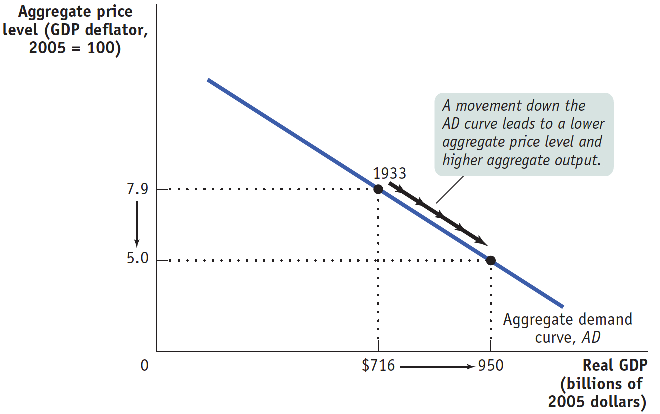
As drawn in Figure 17.1, the aggregate demand curve is downward sloping, indicating a negative relationship between the aggregate price level and the quantity of aggregate output demanded. A higher aggregate price level, other things equal, reduces the quantity of aggregate output demanded; a lower aggregate price level, other things equal, increases the quantity of aggregate output demanded. According to Figure 17.1, if the price level in 1933 had been 5.0 instead of 7.9, the total quantity of domestic final goods and services demanded would have been $950 billion in 2005 dollars instead of $716 billion.

173

The first key question about the aggregate demand curve involves its negative slope.

In Figure 17.1, the curve AD slopes downward. Why? Recall the basic equation of national income accounting:

where C is consumer spending, I is investment spending, G is government purchases of goods and services, X is exports to other countries, and IM is imports. If we measure these variables in constant dollars—that is, in prices of a base year—then C + I + G + X - IM represents the quantity of domestically produced final goods and services demanded during a given period. G is decided by the government, but the other variables are private-sector decisions. To understand why the aggregate demand curve slopes downward, we need to understand why a rise in the aggregate price level reduces C, I, and X - IM.

You might think that the downward slope of the aggregate demand curve is a natural consequence of the law of demand. That is, since the demand curve for any one good is downward-sloping, isn’t it natural that the demand curve for aggregate output is also downward-sloping? This turns out, however, to be a misleading parallel. The demand curve for any individual good shows how the quantity demanded depends on the price of that good, holding the prices of other goods and services constant. The main reason the quantity of a good demanded falls when the price of that good rises—that is, the quantity of a good demanded falls as we move up the demand curve—is that people switch their consumption to other goods and services that have become relatively less expensive.

174

But when we consider movements up or down the aggregate demand curve, we’re considering a simultaneous change in the prices of all final goods and services. Furthermore, changes in the composition of goods and services in consumer spending aren’t relevant to the aggregate demand curve: if consumers decide to buy fewer clothes but more cars, this doesn’t necessarily change the total quantity of final goods and services they demand.

Why, then, does a rise in the aggregate price level lead to a fall in the quantity of all domestically produced final goods and services demanded? There are two main reasons: the wealth effect and the interest rate effect of a change in the aggregate price level.

The Wealth Effect An increase in the aggregate price level, other things equal, reduces the purchasing power of many assets. Consider, for example, someone who has $5,000 in a bank account. If the aggregate price level were to rise by 25%, that $5,000 would buy only as much as $4,000 would have bought previously. With the loss in purchasing power, the owner of that bank account would probably scale back his or her consumption plans. Millions of other people would respond the same way, leading to a fall in spending on final goods and services, because a rise in the aggregate price level reduces the purchasing power of everyone’s bank account.

Correspondingly, a fall in the aggregate price level increases the purchasing power of consumers’ assets and leads to more consumer demand. The wealth effect of a change in the aggregate price level is the change in consumer spending caused by the altered purchasing power of consumers’ assets. Because of the wealth effect, consumer spending, C, falls when the aggregate price level rises, leading to a downward-sloping aggregate demand curve.

The Interest Rate Effect Economists use the term money in its narrowest sense to refer to cash and bank deposits on which people can write checks. People and firms hold money because it reduces the cost and inconvenience of making transactions. An increase in the aggregate price level, other things equal, reduces the purchasing power of a given amount of money holdings. To purchase the same basket of goods and services as before, people and firms now need to hold more money. So, in response to an increase in the aggregate price level, the public tries to increase its money holdings, either by borrowing more or by selling assets such as bonds. This reduces the funds available for lending to other borrowers and drives interest rates up. A rise in the interest rate reduces investment spending because it makes the cost of borrowing higher. It also reduces consumer spending because households save more of their disposable income. So a rise in the aggregate price level depresses investment spending, I, and consumer spending, C, through its effect on the purchasing power of money holdings, an effect known as the interest rate effect of a change in the aggregate price level. This also leads to a downward-sloping aggregate demand curve.

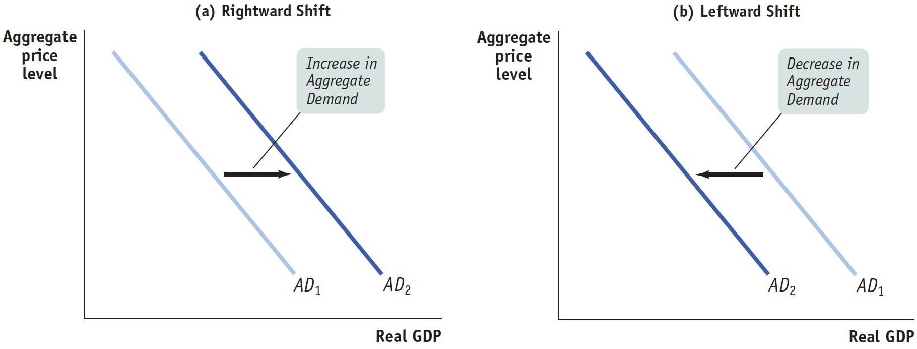
When we introduced the analysis of supply and demand in the market for an individual good, we stressed the importance of the distinction between movements along the demand curve and shifts of the demand curve. The same distinction applies to the aggregate demand curve. Figure 17.1 shows a movement along the aggregate demand curve, a change in the aggregate quantity of goods and services demanded as the aggregate price level changes. But there can also be shifts of the aggregate demand curve, changes in the quantity of goods and services demanded at any given price level, as shown in Figure 17.2. When we talk about an increase in aggregate demand, we mean a shift of the aggregate demand curve to the right, as shown in panel (a) by the shift from AD₁ to AD₂. A rightward shift occurs when the quantity of aggregate output demanded increases at any given aggregate price level. A decrease in aggregate demand means that the AD curve shifts to the left, as in panel (b). A leftward shift implies that the quantity of aggregate output demanded falls at any given aggregate price level.

175

A number of factors can shift the aggregate demand curve. Among the most important factors are changes in expectations, changes in wealth, and the size of the existing stock of physical capital. In addition, both fiscal and monetary policy can shift the aggregate demand curve. All five factors set the spending multiplier process in motion. By causing an initial rise or fall in real GDP, they change disposable income, which leads to additional changes in aggregate spending, which lead to further changes in real GDP, and so on. For an overview of factors that shift the aggregate demand curve, see Table 17.1.

Changes in Expectations Both consumer spending and planned investment spending depend in part on people’s expectations about the future. Consumers base their spending not only on the income they have now but also on the income they expect to have in the future. Firms base their planned investment spending not only on current conditions but also on the sales they expect to make in the future. As a result, changes in expectations can push consumer spending and planned investment spending up or down. If consumers and firms become more optimistic, aggregate spending rises; if they become more pessimistic, aggregate spending falls. In fact, short-run economic forecasters pay careful attention to surveys of consumer and business sentiment. In particular, forecasters watch the Consumer Confidence Index, a monthly measure calculated by the Conference Board, and the Michigan Consumer Sentiment Index, a similar measure calculated by the University of Michigan.

176

Changes in Wealth Consumer spending depends in part on the value of household assets. When the real value of these assets rises, the purchasing power they embody also rises, leading to an increase in aggregate spending. For example, in the 1990s, there was a significant rise in the stock market that increased aggregate demand. And when the real value of household assets falls—for example, because of a stock market crash—the purchasing power they embody is reduced and aggregate demand also falls. The stock market crash of 1929 was a significant factor leading to the Great Depression. Similarly, a sharp decline in real estate values was a major factor depressing consumer spending in 2008.

177

Size of the Existing Stock of Physical Capital Firms engage in planned investment spending to add to their stock of physical capital. Their incentive to spend depends in part on how much physical capital they already have: the more they have, the less they will feel a need to add more, other things equal. The same applies to other types of investment spending—for example, if a large number of houses have been built in recent years, this will depress the demand for new houses and, as a result, will also tend to reduce residential investment spending. In fact, that’s part of the reason for the deep slump in residential investment spending that began in 2006. The housing boom of the previous few years had created an oversupply of houses: by spring 2008, the inventory of unsold houses on the market was equal to more than 11 months of sales, and prices had fallen more than 20% from their peak. This gave the construction industry little incentive to build even more homes.

Government Policies and Aggregate Demand One of the key insights of macroeconomics is that the government can have a powerful influence on aggregate demand and that, in some circumstances, this influence can be used to improve economic performance.

The two main ways the government can influence the aggregate demand curve are through fiscal policy and monetary policy. We’ll briefly discuss their influence on aggregate demand, leaving a full-length discussion for later.

Fiscal Policy Fiscal policy is the use of either government spending—government purchases of final goods and services and government transfers—or tax policy to stabilize the economy. In practice, governments often respond to recessions by increasing spending, cutting taxes, or both. They often respond to inflation by reducing spending or increasing taxes.

The effect of government purchases of final goods and services, G, on the aggregate demand curve is direct because government purchases are themselves a component of aggregate demand. So an increase in government purchases shifts the aggregate demand curve to the right and a decrease shifts it to the left. History’s most dramatic example of how increased government purchases affect aggregate demand was the effect of wartime government spending during World War II. Because of the war, purchases by the U.S. federal government surged 400%. This increase in purchases is usually credited with ending the Great Depression. In the 1990s, Japan used large public works projects—such as government-financed construction of roads, bridges, and dams—in an effort to increase aggregate demand in the face of a slumping economy.

In contrast, changes in either tax rates or government transfers influence the economy indirectly through their effect on disposable income. A lower tax rate means that consumers get to keep more of what they earn, increasing their disposable income. An increase in government transfers also increases consumers’ disposable income. In either case, this increases consumer spending and shifts the aggregate demand curve to the right. A higher tax rate or a reduction in transfers reduces the amount of disposable income received by consumers. This reduces consumer spending and shifts the aggregate demand curve to the left.

Monetary Policy In the next section, we will study the Federal Reserve System and monetary policy in detail. At this point, we just need to note that the Federal Reserve controls monetary policy—the use of changes in the quantity of money or the interest rate to stabilize the economy. We’ve just discussed how a rise in the aggregate price level, by reducing the purchasing power of money holdings, causes a rise in the interest rate. That, in turn, reduces both investment spending and consumer spending.

But what happens if the quantity of money in the hands of households and firms changes? In modern economies, the quantity of money in circulation is largely determined by the decisions of a central bank created by the government. As we’ll learn in more detail later, the Federal Reserve, the U.S. central bank, is a special institution that is neither exactly part of the government nor exactly a private institution. When the central bank increases the quantity of money in circulation, households and firms have more money, which they are willing to lend out. The effect is to drive the interest rate down at any given aggregate price level, leading to higher investment spending and higher consumer spending. That is, increasing the quantity of money shifts the aggregate demand curve to the right. Reducing the quantity of money has the opposite effect: households and firms have less money holdings than before, leading them to borrow more and lend less. This raises the interest rate, reduces investment spending and consumer spending, and shifts the aggregate demand curve to the left.

178