The Demand for Money
Remember that M1, the most commonly used definition of the money supply, consists of currency in circulation (cash), plus checkable bank deposits, plus traveler’s checks. M2, a broader definition of the money supply, consists of M1 plus deposits that can easily be transferred into checkable deposits. You also learned why people hold money—
The Opportunity Cost of Holding Money
Most economic decisions involve trade-
Individuals and firms find it useful to hold some of their assets in the form of money because of the convenience money provides: money can be used to make purchases directly, while other assets can’t. But there is a price to be paid—
As an example of how convenience makes it worth incurring some opportunity costs, consider the fact that even today—
Table 28.1Selected Interest Rates, June 2007
| One- |
5.30% |
| Interest- |
2.30 |
| Currency | 0 |
| Source: Federal Reserve Bank of St. Louis. |
Even holding money in a checking account involves a trade-
Table 28.1 illustrates the opportunity cost of holding money in a specific month. Because interest rates are currently at abnormally low levels, we refer back to June 2007. The first row shows the interest rate on one-
Table 28.1 shows the opportunity cost of holding money at one point in time, but the opportunity cost of holding money changes when the overall level of interest rates changes. Specifically, when the overall level of interest rates falls, the opportunity cost of holding money falls, too.
Short-
Table 28.2 illustrates this point by showing how selected interest rates changed between June 2007 and June 2008, a period when the Federal Reserve was slashing rates in an effort to fight off recession. Between June 2007 and June 2008, the federal funds rate, which is the rate the Fed controls most directly, fell by 3.25 percentage points. The interest rate on one-
Table 28.2Interest Rates and the Opportunity Cost of Holding Money
| June 2007 | June 2008 | |
| Federal funds rate | 5.25% | 2.00% |
| One- |
5.30 | 2.50 |
| Interest- |
2.30 | 1.24 |
| Currency | 0 | 0 |
| CDs minus interest- |
3.00 | 1.26 |
| CDs minus currency | 5.30 | 2.50 |
| Source: Federal Reserve Bank of St. Louis. | ||
Source: Federal Reserve Bank of St. Louis.
Long-Term Interest Rates
Long-Term Interest Rates
Long-
Consider the case of Millie, who has already decided to place $1,000 in CDs for the next two years. However, she hasn’t decided whether to put the money in a one-
You might think that the two-
The same considerations apply to investors deciding between short-
In practice, long-
But as short-
Long-
Table 28.2 contains only short-
The Money Demand Curve
Because the overall level of interest rates affects the opportunity cost of holding money, the quantity of money individuals and firms want to hold, other things equal, is negatively related to the interest rate. In Figure 28.1, the horizontal axis shows the quantity of money demanded and the vertical axis shows the nominal interest rate, r, which you can think of as a representative short-
| Figure 28.1 | The Money Demand Curve |
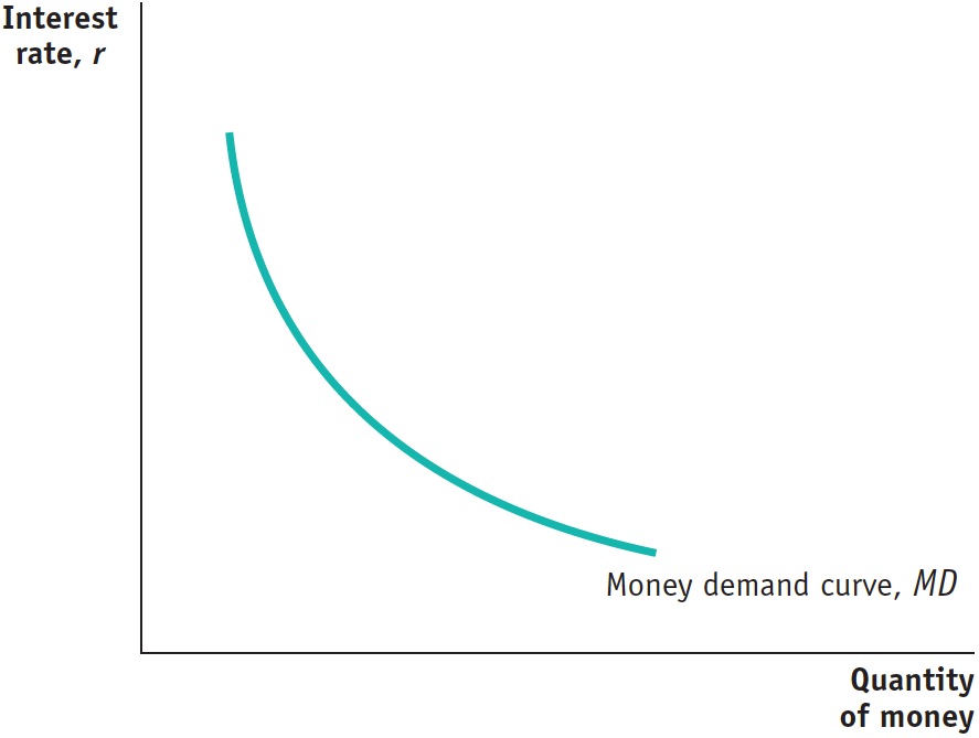
The money demand curve shows the relationship between the quantity of money demanded and the interest rate.
The relationship between the interest rate and the quantity of money demanded by the public is illustrated by the money demand curve, MD, in Figure 28.1. The money demand curve slopes downward because, other things equal, a higher interest rate increases the opportunity cost of holding money, leading the public to reduce the quantity of money it demands. For example, if the interest rate is very low—
AP® Exam Tip
The money market graph is one of the essential graphs you must be able to correctly draw, label, and interpret for the AP® exam. The interest rate measured along the vertical axis is the nominal interest rate.
You might ask why we draw the money demand curve with the interest rate—
Shifts of the Money Demand Curve
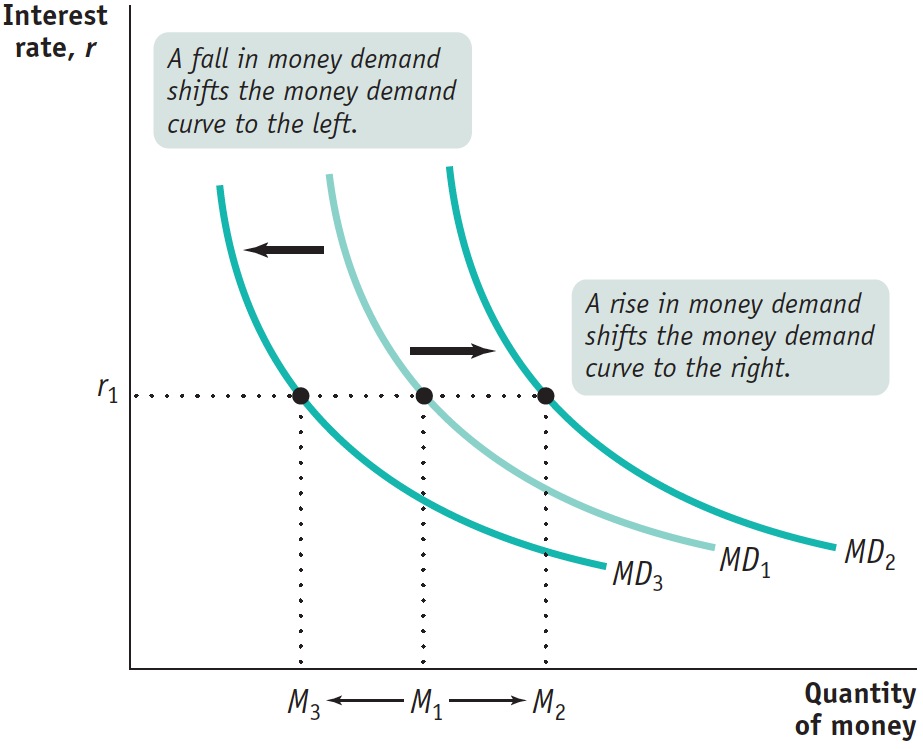
Like the demand curve for an ordinary good, the money demand curve can be shifted by a number of factors. Figure 28.2 shows shifts of the money demand curve: an increase in the demand for money corresponds to a rightward shift of the MD curve, raising the quantity of money demanded at any given interest rate; a fall in the demand for money corresponds to a leftward shift of the MD curve, reducing the quantity of money demanded at any given interest rate. The most important factors causing the money demand curve to shift are changes in the aggregate price level, changes in real GDP, changes in banking technology, and changes in banking institutions.
| Figure 28.2 | Increases and Decreases in the Demand for Money |
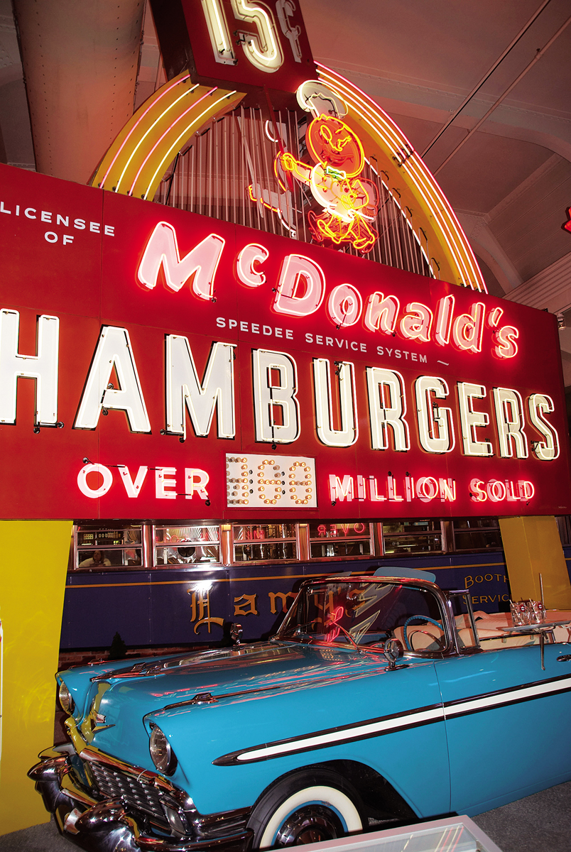
Changes in the Aggregate Price Level Americans keep a lot more cash in their wallets and funds in their checking accounts today than they did in the 1950s. One reason is that they have to if they want to be able to buy anything: almost everything costs more now than it did when you could get a burger, fries, and a drink at McDonald’s for 45 cents and a gallon of gasoline for 29 cents. So higher prices increase the demand for money (a rightward shift of the MD curve), and lower prices decrease the demand for money (a leftward shift of the MD curve).
We can actually be more specific than this: other things equal, the demand for money is proportional to the price level. That is, if the aggregate price level rises by 20%, the quantity of money demanded at any given interest rate, such as r1 in Figure 28.2, also rises by 20%—the movement from M1 to M2. Why? Because if the price of everything rises by 20%, it takes 20% more money to buy the same basket of goods and services. And if the aggregate price level falls by 20%, at any given interest rate the quantity of money demanded falls by 20%—shown by the movement from M1 to M3 at the interest rate r1. As we’ll see later, the fact that money demand is proportional to the price level has important implications for the long-
Changes in Real GDP Households and firms hold money as a way to facilitate purchases of goods and services. The larger the quantity of goods and services they buy, the larger the quantity of money they will want to hold at any given interest rate. So an increase in real GDP—
AP® Exam Tip
Changes in the aggregate price level, real GDP, technology, and banking institutions shift the money demand curve. On the AP® exam you may be given scenarios in which you must determine the direction of a shift in this curve.
Changes in Technology There was a time, not so long ago, when withdrawing cash from a bank account required a visit during the bank’s hours of operation. Since most people tried to do their banking during lunch hour, they often found themselves standing in line. So people limited the number of times they needed to withdraw funds by keeping substantial amounts of cash on hand. Not surprisingly, this tendency diminished greatly with the advent of ATMs in the 1970s. As a result, the demand for money fell and the money demand curve shifted leftward.
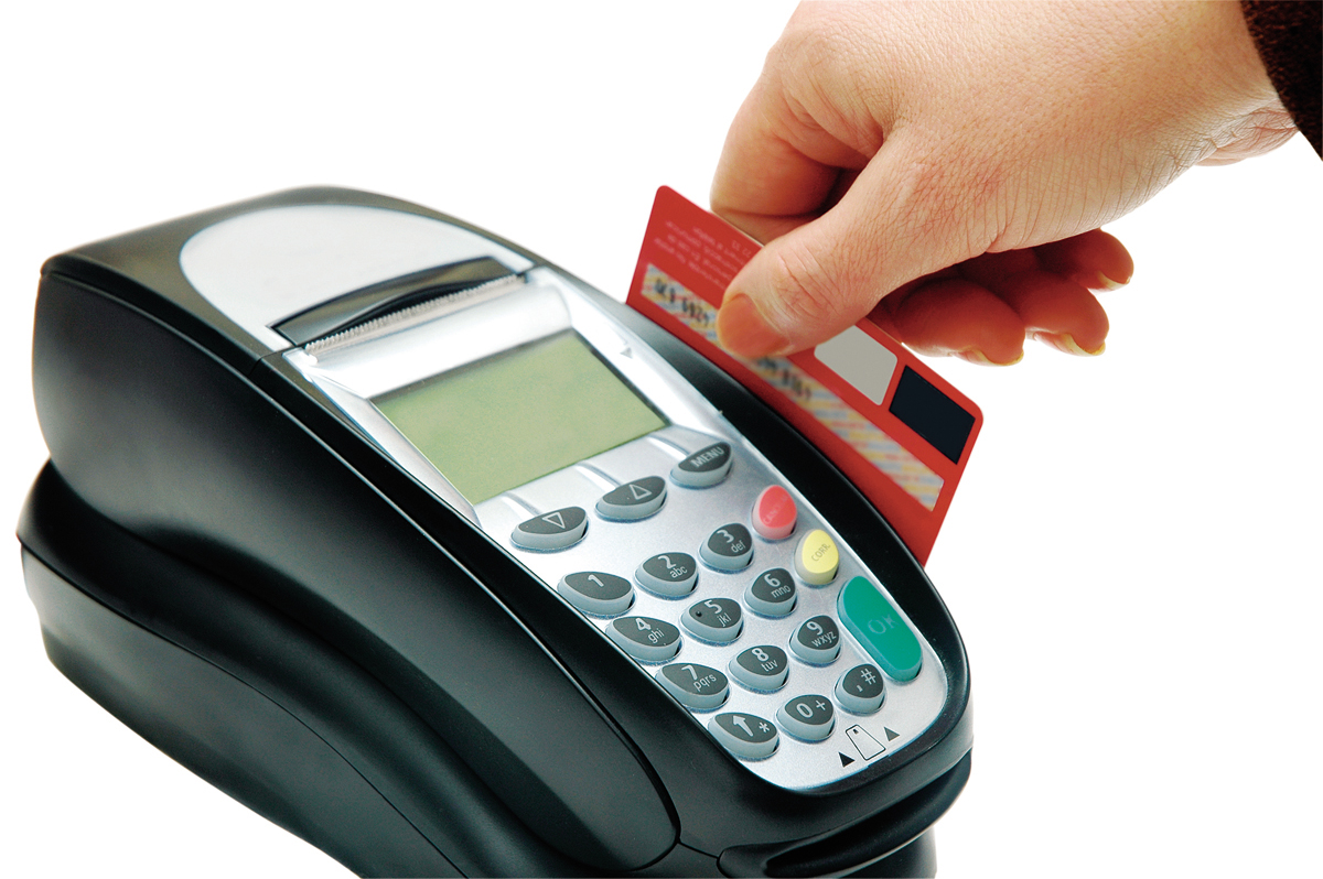
These events illustrate how changes in technology can affect the demand for money. In general, advances in information technology have tended to reduce the demand for money by making it easier for the public to make purchases without holding significant sums of money. ATMs are only one example of how changes in technology have altered the demand for money. The ability of stores to process credit card and debit card transactions via the Internet has widened their acceptance and similarly reduced the demand for cash.
Changes in Institutions Changes in institutions can increase or decrease the demand for money. For example, until Regulation Q was eliminated in 1980, U.S. banks weren’t allowed to offer interest on checking accounts. So the interest you would forgo by holding funds in a checking account instead of an interest-
Money and Interest Rates
The Federal Open Market Committee decided today to lower its target for the federal funds rate 75 basis points to 2¼ percent.
Recent information indicates that the outlook for economic activity has weakened further. Growth in consumer spending has slowed and labor markets have softened. Financial markets remain under considerable stress, and the tightening of credit conditions and the deepening of the housing contraction are likely to weigh on economic growth over the next few quarters.
So read the beginning of a press release from the Federal Reserve issued on March 18, 2008. (A basis point is equal to 0.01 percentage point. So the statement implies that the Fed lowered the target from 3% to 2.25%.) Remember that the federal funds rate is the rate at which banks lend reserves to each other to meet the required reserve ratio. As the statement implies, at each of its eight-
As we’ve already seen, other short-
How does the Fed go about achieving a target federal funds rate? And more to the point, how is the Fed able to affect interest rates at all?
The Equilibrium Interest Rate
According to the liquidity preference model of the interest rate, the interest rate is determined by the supply and demand for money.
The money supply curve shows the relationship between the quantity of money supplied and the interest rate.
Recall that, for simplicity, we’ve assumed that there is only one interest rate paid on nonmonetary financial assets, both in the short run and in the long run. To understand how the interest rate is determined, consider Figure 28.3, which illustrates the liquidity preference model of the interest rate; this model says that the interest rate is determined by the supply and demand for money in the market for money. Figure 28.3 combines the money demand curve, MD, with the money supply curve, MS, which shows the relationship between the quantity of money supplied by the Federal Reserve and the interest rate.
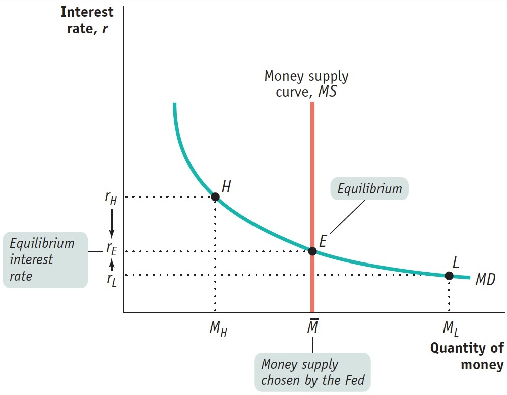
| Figure 28.3 | Equilibrium in the Money Market |
 . The money market is in equilibrium at the interest rate rE: the quantity of money demanded by the public is equal to , the quantity of money supplied. At a point such as L, the interest rate, rL, is below rE and the corresponding quantity of money demanded, ML, exceeds the money supply, . In an attempt to shift their wealth out of nonmoney interest-. In an attempt to shift out of money holdings into nonmoney interest-
The Federal Reserve can increase or decrease the money supply: it usually does this through open-. The money market equilibrium is at E, where MS and MD cross. At this point the quantity of money demanded equals the money supply, , leading to an equilibrium interest rate of rE.
To understand why rE is the equilibrium interest rate, consider what happens if the money market is at a point like L, where the interest rate, rL, is below rE. At rL the public wants to hold the quantity of money ML, an amount larger than the actual money supply, . This means that at point L, the public wants to shift some of its wealth out of interest-
Now consider what happens if the money market is at a point such as H in Figure 28.3, where the interest rate rH is above rE. In that case the quantity of money demanded, MH, is less than the quantity of money supplied, . Correspondingly, the quantity of interest-. Again, the interest rate will end up at rE.
Two Models of the Interest Rate
Here we have developed the liquidity preference model of the interest rate. In this model, the equilibrium interest rate is the rate at which the quantity of money demanded equals the quantity of money supplied in the money market. This model is different from, but consistent with, another model known as the loanable funds model of the interest rate, which is developed in the next module. In the loanable funds model, we will see that the interest rate matches the quantity of loanable funds supplied by savers with the quantity of loanable funds demanded for investment spending.