Chapter Introduction
MODULE 29
The Market for Loanable Funds

In this Module, you will learn to:
• Describe how the loanable funds market matches savers and investors
• Identify the determinants of supply and demand in the loanable funds market
• Explain how the two models of interest rates can be reconciled
The Market for Loanable Funds
Recall that, for the economy as a whole, savings always equals investment spending. In a closed economy, savings is equal to national savings. In an open economy, savings is equal to national savings plus capital inflow. At any given time, however, savers, the people with funds to lend, are usually not the same as borrowers, the people who want to borrow to finance their investment spending. How are savers and borrowers brought together?
Savers and borrowers are matched up with one another in much the same way producers and consumers are matched up: through markets governed by supply and demand. In the circular-
The loanable funds market is a hypothetical market that brings together those who want to lend money and those who want to borrow money.
The Equilibrium Interest Rate There are a large number of different financial markets in the financial system, such as the bond market and the stock market. However, economists often work with a simplified model in which they assume that there is just one market that brings together those who want to lend money (savers) and those who want to borrow money (firms with investment spending projects). This hypothetical market is known as the loanable funds market. The price that is determined in the loanable funds market is the interest rate, denoted by r. It is the return a lender receives for allowing borrowers the use of a dollar for one year, calculated as a percentage of the amount borrowed.
Recall that in the money market, the nominal interest rate is of central importance and always serves as the “price” measured on the vertical axis. The interest rate in the loanable funds market can be measured in either real or nominal terms—
The rate of return on a project is the profit earned on the project expressed as a percentage of its cost.
We should also note at this point that, in reality, there are many different kinds of nominal interest rates because there are many different kinds of loans—

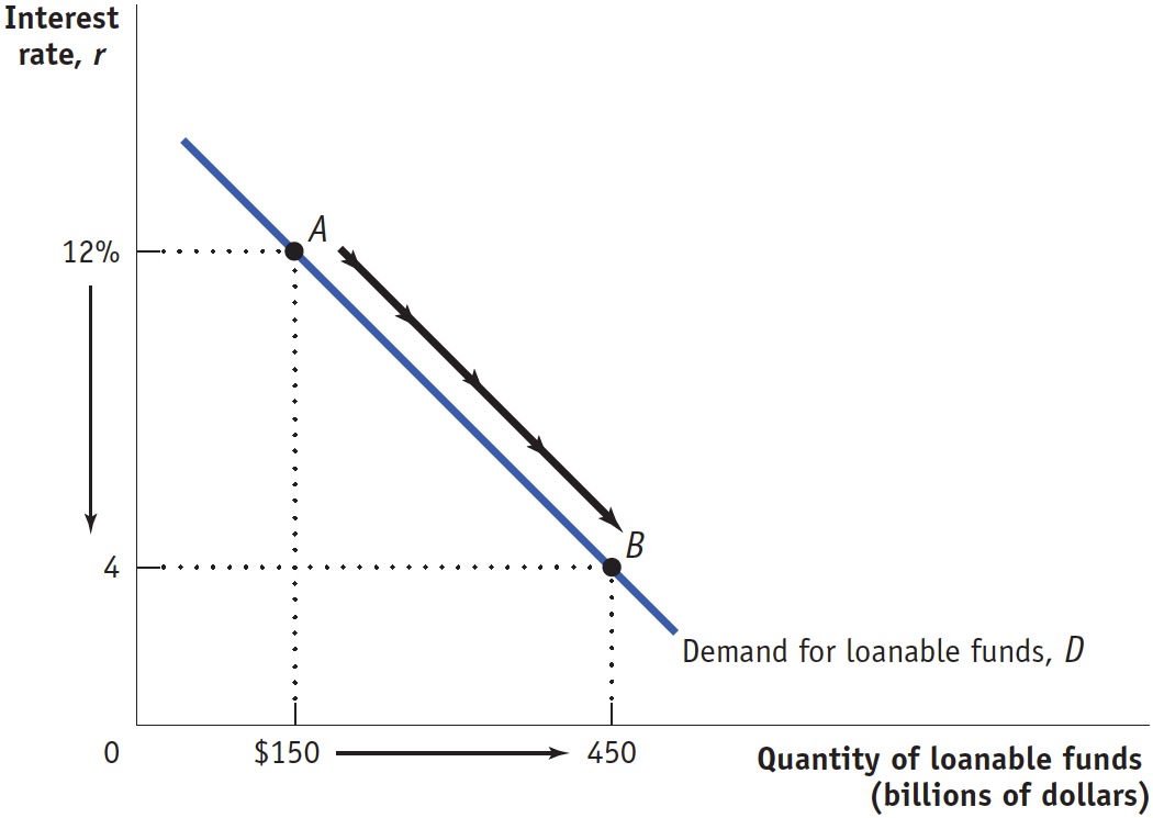
| Figure 29.1 | The Demand for Loanable Funds |
For example, a project that costs $300,000 and produces revenue of $315,000 provides a rate of return of [($315,000 – $300,000)/$300,000] × 100 = 5%.
AP® Exam Tip
When expectations about the future inflation rate remain unchanged, the real interest rate and the nominal interest rate rise and fall together, and either rate can appear on the vertical axis of the loanable funds graph. We use the nominal interest rate here for comparability with the money market graph. If a question asks you to draw conclusions about the real interest rate on the basis of the loanable funds graph, simply label the vertical axis “real interest rate.”
A business will want a loan when the rate of return on its project is greater than or equal to the interest rate. So, for example, at an interest rate of 12%, only businesses with projects that yield a rate of return greater than or equal to 12% will want a loan. A business will not pay 12% interest to fund a project with a 5% rate of return. The demand curve in Figure 29.1 shows that if the interest rate is 12%, businesses will want to borrow $150 billion (point A); if the interest rate is only 4%, businesses will want to borrow a larger amount, $450 billion (point B). That’s a consequence of our assumption that the demand curve slopes downward: the lower the interest rate, the larger the total quantity of loanable funds demanded. Why do we make that assumption? Because, in reality, the number of potential investment projects that yield at least 4% is always greater than the number that yield at least 12%.
AP® Exam Tip
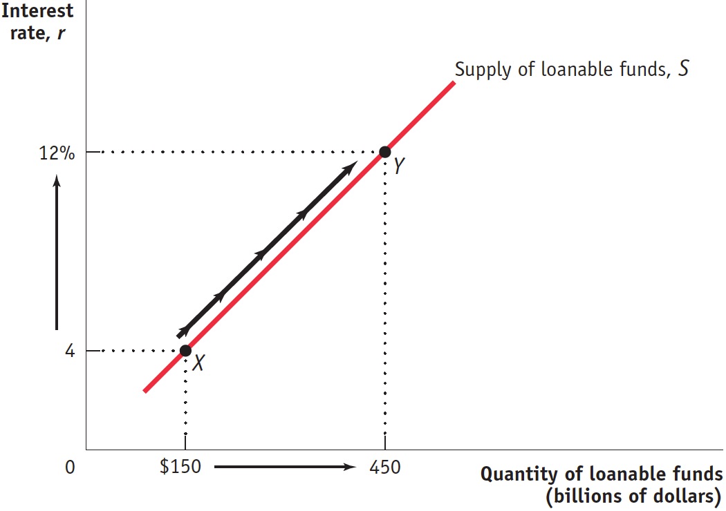
The loanable funds graph is another essential graph for the AP® exam. The incentive to lend money is higher when the interest rate is higher, so the supply curve for loanable funds has an upward slope.
Figure 29.2 shows the hypothetical supply of loanable funds. Again, the interest rate plays the same role that the price plays in ordinary supply and demand analysis. Savers incur an opportunity cost when they lend to a business; the funds could instead be spent on consumption—
| Figure 29.2 | The Supply of Loanable Funds |
The equilibrium interest rate is the interest rate at which the quantity of loanable funds supplied equals the quantity of loanable funds demanded. As you can see in Figure 29.3, the equilibrium interest rate, rE, and the total quantity of lending, QE, are determined by the intersection of the supply and demand curves, at point E. Here, the equilibrium interest rate is 8%, at which $300 billion is lent and borrowed. Investment spending projects with a rate of return of 8% or more are funded; projects with a rate of return of less than 8% are not. Correspondingly, only lenders who are willing to accept an interest rate of 8% or less will have their offers to lend funds accepted.
| Figure 29.3 | Equilibrium in the Loanable Funds Market |
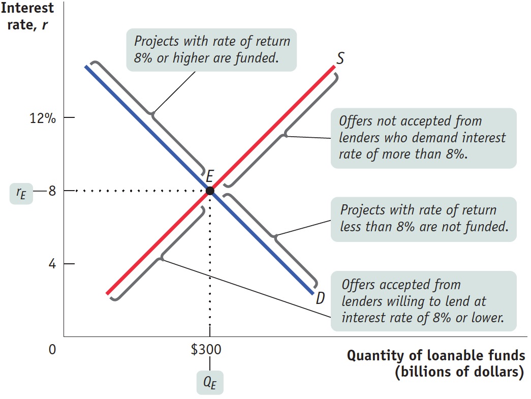
Figure 29.3 shows how the market for loanable funds matches up desired savings with desired investment spending: in equilibrium, the quantity of funds that savers want to lend is equal to the quantity of funds that firms want to borrow. The figure also shows that this match-
Before we get to that, however, let’s look at how the market for loanable funds responds to shifts of demand and supply.
Shifts of the Demand for Loanable Funds The equilibrium interest rate changes when there are shifts of the demand curve for loanable funds, the supply curve for loanable funds, or both. Let’s start by looking at the causes and effects of changes in demand.
The factors that can cause the demand curve for loanable funds to shift include the following:
Changes in perceived business opportunities. A change in beliefs about the rate of return on investment spending can increase or reduce the amount of desired spending at any given interest rate. For example, during the 1990s there was great excitement over the business possibilities created by the Internet, which had just begun to be widely used. As a result, businesses rushed to buy computer equipment, put fiber-
optic cables in the ground, and so on. This shifted the demand for loanable funds to the right. By 2001, the failure of many dot- com businesses led to disillusionment with technology- related investment; this shifted the demand for loanable funds back to the left. Changes in the government’s borrowing. Governments that run budget deficits are major sources of the demand for loanable funds. As a result, changes in the budget deficit can shift the demand curve for loanable funds. For example, between 2000 and 2003, as the U.S. federal government went from a budget surplus to a budget deficit, net federal borrowing went from minus $189 billion—
that is, in 2000 the federal government was actually providing loanable funds to the market because it was paying off some of its debt— to plus $416 billion because in 2003 the government had to borrow large sums to pay its bills. This change in the federal budget position had the effect, other things equal, of shifting the demand curve for loanable funds to the right.

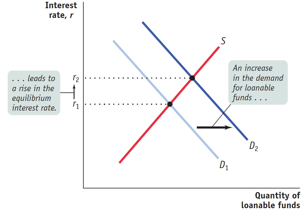
Figure 29.4 shows the effects of an increase in the demand for loanable funds. S is the supply of loanable funds, and D1 is the initial demand curve. The initial equilibrium interest rate is r1. An increase in the demand for loanable funds means that the quantity of funds demanded rises at any given interest rate, so the demand curve shifts rightward to D2. As a result, the equilibrium interest rate rises to r2.
| Figure 29.4 | An Increase in the Demand for Loanable Funds |
Crowding out occurs when a government deficit drives up the interest rate and leads to reduced investment spending.
The fact that, other things equal, an increase in the demand for loanable funds leads to a rise in the interest rate has one especially important implication: beyond concern about repayment, there are other reasons to be wary of government budget deficits. As we’ve already seen, an increase in the government’s deficit shifts the demand curve for loanable funds to the right, which leads to a higher interest rate. If the interest rate rises, businesses will cut back on their investment spending. So a rise in the government budget deficit tends to reduce overall investment spending. Economists call the negative effect of government budget deficits on investment spending crowding out. The threat of crowding out is a key source of concern about persistent budget deficits.
Shifts of the Supply of Loanable Funds Like the demand for loanable funds, the supply of loanable funds can shift. Among the factors that can cause the supply of loanable funds to shift are the following:
Changes in private saving behavior. A number of factors can cause the level of private savings to change at any given rate of interest. For example, between 2000 and 2006 rising home prices in the United States made many homeowners feel richer, making them willing to spend more and save less. This had the effect of shifting the supply of loanable funds to the left. The drop in home prices between 2006 and 2009 had the opposite effect, shifting the supply of loanable funds to the right.
Changes in capital inflows. Capital flows into a country can change as investors’ perceptions of that country change. For example, Brazil experienced large capital inflows during much of the last decade because international investors believed that years of economic reforms made it a safe place to put their funds. As we’ve already seen, the United States has received large capital inflows in recent years, with much of the money coming from China and the Middle East. Those inflows helped fuel a big increase in residential investment spending—
newly constructed homes— from 2003 to 2006. As a result of the worldwide slump, those inflows trailed off in 2008 and remained relatively low through early 2014.

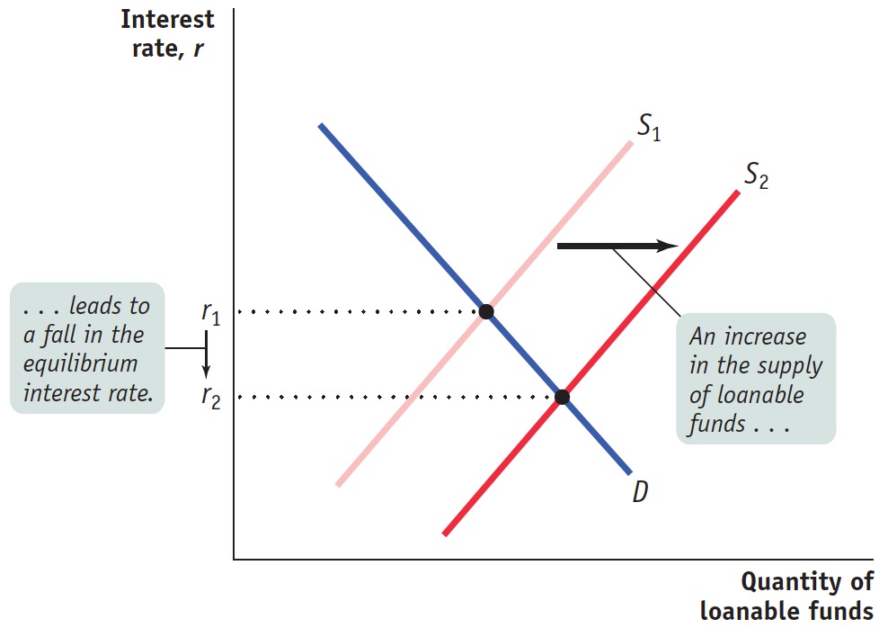
Figure 29.5 shows the effects of an increase in the supply of loanable funds. D is the demand for loanable funds, and S1 is the initial supply curve. The initial equilibrium interest rate is r1. An increase in the supply of loanable funds means that the quantity of funds supplied rises at any given interest rate, so the supply curve shifts rightward to S2. As a result, the equilibrium interest rate falls to r2.
| Figure 29.5 | An Increase in the Supply of Loanable Funds |
Inflation and Interest Rates Anything that shifts either the supply of loanable funds curve or the demand for loanable funds curve changes the interest rate. Historically, major changes in interest rates have been driven by many factors, including changes in government policy and technological innovations that created new investment opportunities. However, arguably the most important factor affecting interest rates over time—
To understand the effect of expected inflation on interest rates, recall our discussion in Module 14 of the way inflation creates winners and losers—
Real interest rate = Nominal interest rate – Inflation rate
The true cost of borrowing is the real interest rate, not the nominal interest rate. To see why, suppose a firm borrows $10,000 for one year at a 10% nominal interest rate. At the end of the year, it must repay $11,000—
Similarly, the true payoff to lending is the real interest rate, not the nominal rate. The bank that makes the one-
The expectations of borrowers and lenders about future inflation rates are normally based on recent experience. In the late 1970s, after a decade of high inflation, borrowers and lenders expected future inflation to be high. By the late 1990s, after a decade of fairly low inflation, borrowers and lenders expected future inflation to be low. And these changing expectations about future inflation had a strong effect on the nominal interest rate, largely explaining why interest rates were much lower in the early years of the twenty-
Let’s look at how changes in the expected future rate of inflation are reflected in the loanable funds model. In Figure 29.6, the curves S0 and D0 show the supply of and demand for loanable funds given that the expected future rate of inflation is 0%. In that case, equilibrium is at E0 and the equilibrium nominal interest rate is 4%. Because expected future inflation is 0%, the equilibrium expected real interest rate over the life of the loan, the real interest rate expected by borrowers and lenders when the loan is contracted, is also 4%.
| Figure 29.6 | The Fisher Effect |
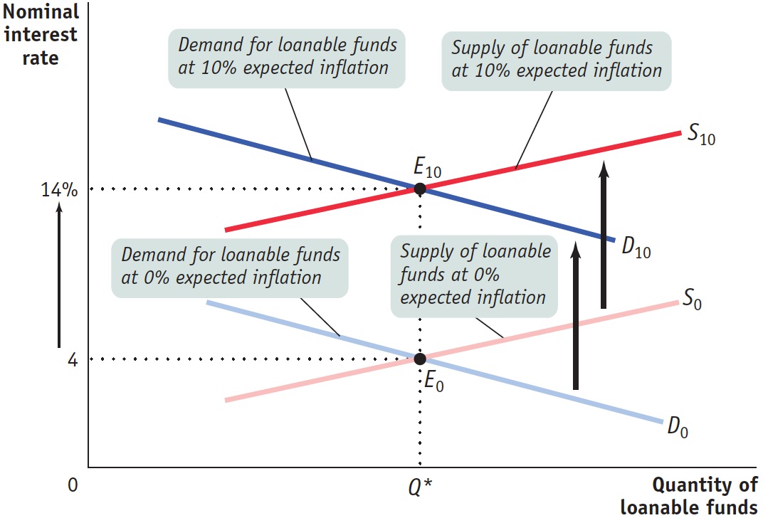
Now suppose that the expected future inflation rate rises to 10%. The demand curve for funds shifts upward to D10: borrowers are now willing to borrow as much at a nominal interest rate of 14% as they were previously willing to borrow at 4%. That’s because with a 10% inflation rate, a borrower who pays a 14% nominal interest rate pays a 4% real interest rate. Similarly, the supply curve of funds shifts upward to S10: lenders require a nominal interest rate of 14% to persuade them to lend as much as they would previously have lent at 4%. That’s because with a 10% inflation rate, a lender who receives a 14% nominal interest rate receives a 4% real interest rate. The new equilibrium is at E10: the result of an increase in the expected future inflation rate from 0% to 10% is that the equilibrium nominal interest rate rises from 4% to 14%.
According to the Fisher effect, an increase in expected future inflation drives up the nominal interest rate by the same number of percentage points, leaving the expected real interest rate unchanged.
This situation can be summarized as a general principle, named the Fisher effect after the American economist Irving Fisher, who proposed it in 1930: an increase in expected inflation drives up the nominal interest rate by the same number of percentage points, leaving the expected real interest rate unchanged. The central point is that both lenders and borrowers base their decisions on the expected real interest rate. As a result, a change in the expected rate of inflation does not affect the equilibrium quantity of loanable funds or the expected real interest rate; all it affects is the equilibrium nominal interest rate.