Moderate Inflation and Disinflation
The governments of wealthy, politically stable countries like the United States and Britain don’t find themselves forced to print money to pay their bills. Yet over the past 40 years, both countries, along with a number of other nations, have experienced uncomfortable episodes of inflation. In the United States, the inflation rate peaked at 13% in 1980. In Britain, the inflation rate reached 26% in 1975. Why did policy makers allow this to happen?
Cost-push inflation is inflation that is caused by a significant increase in the price of an input with economy-wide importance.
Using the aggregate demand and supply model, we can see that there are two possible changes that can lead to an increase in the aggregate price level: a decrease in aggregate supply or an increase in aggregate demand. Inflation that is caused by a significant increase in the price of an input with economy-wide importance is called cost-push inflation. For example, it is argued that the oil crisis in the 1970s led to an increase in energy prices in the United States, causing a leftward shift of the aggregate supply curve, increasing the aggregate price level. However, aside from crude oil, it is difficult to think of examples of inputs with economy-wide importance that experience significant price increases.
Demand-pull inflation is inflation that is caused by an increase in aggregate demand.
Inflation that is caused by an increase in aggregate demand is known as demand-pull inflation. When a rightward shift of the aggregate demand curve leads to an increase in the aggregate price level, the economy experiences demand-pull inflation. This is sometimes described by the phrase “too much money chasing too few goods,” which means that the aggregate demand for goods and services is outpacing the aggregate supply and driving up the prices of goods.
Page 324
In the short run, policies that produce a booming economy also tend to lead to higher inflation, and policies that reduce inflation tend to depress the economy. This creates both temptations and dilemmas for governments.
AP® Exam Tip
Make sure you can graph and explain cost-push inflation and demand-pull inflation, as these are both tested frequently on the AP® exam. Remember that cost-push inflation is a leftward shift of AS and demand-pull inflation is a rightward shift of AD.
Imagine yourself as a politician facing an election in a year, and suppose that inflation is fairly low at the moment. You might well be tempted to pursue expansionary policies that will push the unemployment rate down, as a way to please voters, even if your economic advisers warn that this will eventually lead to higher inflation. You might also be tempted to find different economic advisers, who will tell you not to worry: in politics, as in ordinary life, wishful thinking often prevails over realistic analysis.
Conversely, imagine yourself as a politician in an economy suffering from inflation. Your economic advisers will probably tell you that the only way to bring inflation down is to push the economy into a recession, which will lead to temporarily higher unemployment. Are you willing to pay that price? Maybe not.
This political asymmetry—inflationary policies often produce short-term political gains, but policies to bring inflation down carry short-term political costs—explains how countries with no need to impose an inflation tax sometimes end up with serious inflation problems. For example, that 26% rate of inflation in Britain was largely the result of the British government’s decision in 1971 to pursue highly expansionary monetary and fiscal policies. Politicians disregarded warnings that these policies would be inflationary and were extremely reluctant to reverse course even when it became clear that the warnings had been correct.
But why do expansionary policies lead to inflation? To answer that question, we need to look first at the relationship between output and unemployment. Then we’ll add inflation to the story in Module 34.
The Output Gap and the Unemployment Rate
Earlier we introduced the concept of potential output, the level of real GDP that the economy would produce once all prices had fully adjusted. Potential output typically grows steadily over time, reflecting long-run growth. However, as we learned from the aggregate demand–aggregate supply model, actual aggregate output fluctuates around potential output in the short run: a recessionary gap arises when actual aggregate output falls short of potential output; an inflationary gap arises when actual aggregate output exceeds potential output. Recall that the percentage difference between the actual level of real GDP and potential output is called the output gap. A positive or negative output gap occurs when an economy is producing more or less than what would be “expected” because all prices have not yet adjusted. And, as we’ve learned, wages are the prices in the labor market.
Meanwhile, we learned that the unemployment rate is composed of cyclical unemployment and natural unemployment, the portion of the unemployment rate unaffected by the business cycle. So there is a relationship between the unemployment rate and the output gap. This relationship is defined by two rules:
When actual aggregate output is equal to potential output, the actual unemployment rate is equal to the natural rate of unemployment.
When the output gap is positive (an inflationary gap), the unemployment rate is below the natural rate. When the output gap is negative (a recessionary gap), the unemployment rate is above the natural rate.
In other words, fluctuations of aggregate output around the long-run trend of potential output correspond to fluctuations of the unemployment rate around the natural rate.
This makes sense. When the economy is producing less than potential output—when the output gap is negative—it is not making full use of its productive resources. Among the resources that are not fully used is labor, the economy’s most important resource. So we would expect a negative output gap to be associated with unusually high unemployment. Conversely, when the economy is producing more than potential output, it is temporarily using resources at higher-than-normal rates. With this positive output gap, we would expect to see lower-than-normal unemployment.
Page 325
Figure 33.3 confirms this rule. Panel (a) shows the actual and natural rates of unemployment, as estimated by the Congressional Budget Office (CBO). Panel (b) shows two series. One is cyclical unemployment: the difference between the actual unemployment rate and the CBO estimate of the natural rate of unemployment, measured on the left. The other is the CBO estimate of the output gap, measured on the right. To make the relationship clearer, the output gap series is inverted—shown upside down—so that the line goes down if actual output rises above potential output and up if actual output falls below potential output. As you can see, the two series move together quite closely, showing the strong relationship between the output gap and cyclical unemployment. Years of high cyclical unemployment, like 1982 or 2009, were also years of a strongly negative output gap. Years of low cyclical unemployment, like the late 1960s or 2000, were years of a strongly positive output gap.
| Figure 33.3 | Cyclical Unemployment and the Output Gap |
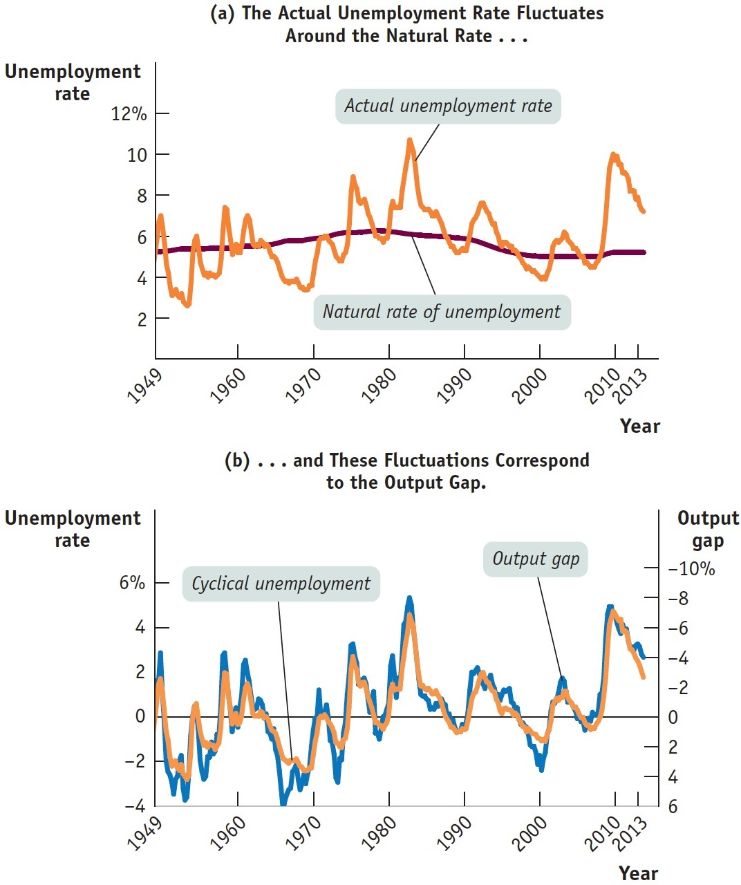
Figure 33.3: Cyclical Unemployment and the Output GapPanel (a) shows the actual U.S. unemployment rate from 1949 to 2013, together with the Congressional Budget Office (CBO) estimate of the natural rate of unemployment. The actual rate fluctuates around the natural rate, often for extended periods. Panel (b) shows cyclical unemployment—the difference between the actual unemployment rate and the natural rate of unemployment—and the output gap, also estimated by the CBO. The unemployment rate is measured on the left vertical axis, and the output gap is measured with an inverted scale on the right vertical axis. With an inverted scale, it moves in the same direction as the unemployment rate: when the output gap is positive, the actual unemployment rate is below its natural rate; when the output gap is negative, the actual unemployment rate is above its natural rate. The two series track one another closely, showing the strong relationship between the output gap and cyclical unemployment.
Sources: Congressional Budget Office; Bureau of Labor Statistics; Bureau of Economic Analysis.