Inflation and Unemployment: The Phillips Curve
Tom Bonaventure/ Photographer’s Choice RF/Getty Images
34Inflation and Unemployment: The Phillips Curve
In this Module, you will learn to:
• Use the Phillips curve to show the nature of the short-run trade-off between inflation and unemployment
• Explain why there is no long-run trade-off between inflation and unemployment
• Discuss why expansionary policies are limited due to the effects of expected inflation
• Explain why even moderate levels of inflation can be hard to end
• Identify the problems with deflation that lead policy makers to prefer a low but positive inflation rate
The Short-Run Phillips Curve
We’ve just seen that expansionary policies lead to a lower unemployment rate. Our next step in understanding the temptations and dilemmas facing governments is to show that there is a short-run trade-off between unemployment and inflation—lower unemployment tends to lead to higher inflation, and vice versa. The key concept is that of the Phillips curve.
The origins of this concept lie in a famous 1958 paper by the New Zealand–born economist Alban W. H. Phillips. Looking at historical data for Britain, he found that when the unemployment rate was high, the wage rate tended to fall, and when the unemployment rate was low, the wage rate tended to rise. Using data from Britain, the United States, and elsewhere, other economists soon found a similar apparent relationship between the unemployment rate and the rate of inflation—that is, the rate of change in the aggregate price level. For example, Figure 34.1 shows the U.S. unemployment rate and the rate of consumer price inflation over each subsequent year from 1955 to 1968, with each dot representing one year’s data.
| Figure 34.1 | Unemployment and Inflation, 1955–1968 |
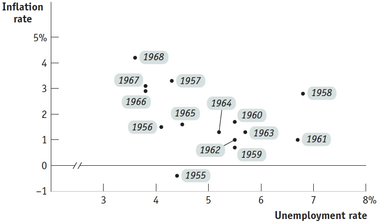
Figure 34.1: Unemployment and Inflation, 1955–1968Each dot shows the average U.S. unemployment rate for one year and the percentage increase in the consumer price index over the subsequent year. Data like this lay behind the initial concept of the Phillips curve.
Source: Bureau of Labor Statistics.
The short-run Phillips curve represents the negative short-run relationship between the unemployment rate and the inflation rate.
Looking at evidence like Figure 34.1, many economists concluded that there is a negative short-run relationship between the unemployment rate and the inflation rate, represented by the short-run Phillips curve, or SRPC. (We’ll explain the difference between the short-run and the long-run Phillips curve soon.) Figure 34.2 shows a hypothetical short-run Phillips curve.
| Figure 34.2 | The Short-Run Phillips Curve |
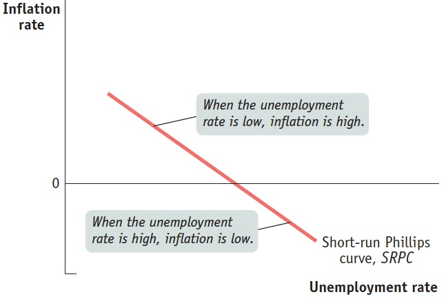
Figure 34.2: The Short-Run Phillips CurveThe short-run Phillips curve, SRPC, slopes downward because the relationship between the unemployment rate and the inflation rate is negative.
Page 329
We can better understand the shape of the Phillips curve by examining its ties to the AD–AS model. Panel (a) of Figure 34.3 shows how changes in the aggregate price level and the output gap depend on changes in aggregate demand. Assume that in year 1 the aggregate demand curve is AD1, the long-run aggregate supply curve is LRAS, and the short-run aggregate supply curve is SRAS. The initial macroeconomic equilibrium is at E1, where the price level is 100 and real GDP is $10 trillion. Notice that at E1 real GDP is equal to potential output, so the output gap is zero.
| Figure 34.3 | The AD–AS Model and the Short-Run Phillips Curve |
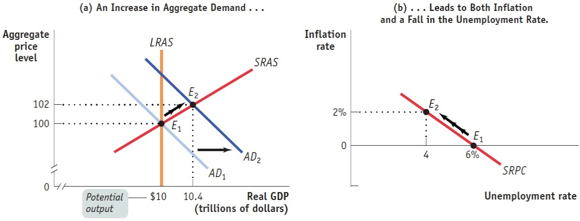
Figure 34.3: The AD–AS Model and the Short-Run Phillips CurveShifts in aggregate demand lead to movements along the Phillips curve. In panel (a), the economy is initially in equilibrium at E1, with the aggregate price level at 100 and aggregate output at $10 trillion, which we assume is potential output. Now consider two possibilities. If the aggregate demand curve remains at AD1, there is an output gap of zero and 0% inflation. If the aggregate demand curve shifts out to AD2, the positive output gap reduces unemployment to 4%, and inflation rises to 2%. Assuming that the natural rate of unemployment is 6%, the implications for unemployment and inflation are shown in panel (b): with aggregate demand at AD1, 6% unemployment and 0% inflation will result; if aggregate demand increases to AD2, 4% unemployment and 2% inflation will result.
Now consider what happens if aggregate demand shifts rightward to AD2 and the economy moves to E2. At E2, Real GDP is $10.4 trillion, $0.4 trillion more than potential output—forming a 4% output gap. Meanwhile, at E2 the aggregate price level has risen to 102—a 2% increase. So panel (a) indicates that in this example a zero output gap is associated with zero inflation and a 4% output gap is associated with 2% inflation.
Panel (b) shows what this implies for the relationship between unemployment and inflation: an increase in aggregate demand leads to a fall in the unemployment rate and an increase in the inflation rate. Assume that the natural rate of unemployment is 6% and that a rise of 1 percentage point in the output gap causes a fall of ½ percentage point in the unemployment rate (this is a predicted relationship between the output gap and the unemployment rate known as Okun’s law). Then E1 and E2 in panel (a) correspond to E1 and E2 in panel (b). At E1, the unemployment rate is 6% and the inflation rate is 0%. At E2, the unemployment rate is 4%, because an output gap of 4% reduces the unemployment rate by 4% × 0.5 = 2% below its natural rate of 6%—and the inflation rate is 2%. This is an example of the negative relationship between unemployment and inflation.
Page 330
Going in the other direction, a decrease in aggregate demand leads to a rise in the unemployment rate and a fall in the inflation rate. This corresponds to a movement downward and to the right along the short-run Phillips curve. So, other things equal, increases and decreases in aggregate demand result in movements to the left and right along the short-run Phillips curve.
Changes in aggregate supply also affect the Phillips curve. Previously, we discussed the effect of supply shocks, such as sudden changes in the price of oil, that shift the short-run aggregate supply curve. Such shocks shift the short-run Phillips curve: surging oil prices were an important factor in the inflation of the 1970s and also played an important role in the acceleration of inflation in 2007–2008. In general, a negative supply shock shifts SRPC up, as the inflation rate increases for every level of the unemployment rate, and a positive supply shock shifts it down as the inflation rate falls for every level of the unemployment rate. Both outcomes are shown in Figure 34.4.
| Figure 34.4 | The Short-Run Phillips Curve and Supply Shocks |
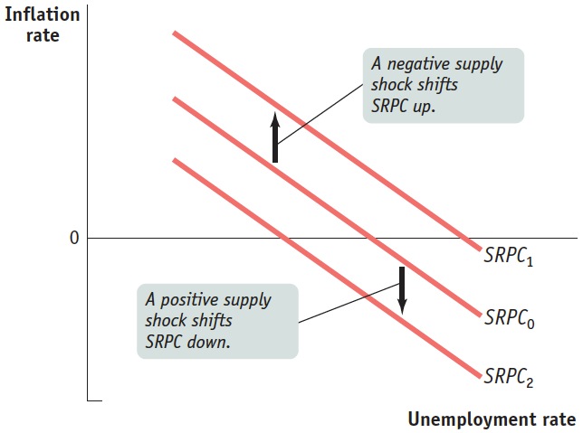
Figure 34.4: The Short-Run Phillips Curve and Supply ShocksA negative supply shock shifts the SRPC up, and a positive supply shock shifts the SRPC down.
But supply shocks are not the only factors that can shift the Phillips curve. In the early 1960s, Americans had little experience with inflation, as inflation rates had been low for decades. But by the late 1960s, after inflation had been steadily increasing for a number of years, Americans had come to expect future inflation. In 1968 two economists—Milton Friedman of the University of Chicago and Edmund Phelps of Columbia University—independently set forth a crucial hypothesis: that expectations about future inflation directly affect the present inflation rate. Today most economists accept that the expected inflation rate—the rate of inflation that employers and workers expect in the near future—is the most important factor, other than the unemployment rate, affecting inflation.
Inflation Expectations and the Short-Run Phillips Curve
Page 331
The expected rate of inflation is the rate that employers and workers expect in the near future. One of the crucial discoveries of modern macroeconomics is that changes in the expected rate of inflation affect the short-run trade-off between unemployment and inflation and shift the short-run Phillips curve.
Why do changes in expected inflation affect the short-run Phillips curve? Put yourself in the position of a worker or employer about to sign a contract setting the worker’s wages over the next year. For a number of reasons, the wage rate they agree to will be higher if everyone expects high inflation (including rising wages) than if everyone expects prices to be stable. The worker will want a wage rate that takes into account future declines in the purchasing power of earnings. He or she will also want a wage rate that won’t fall behind the wages of other workers. And the employer will be more willing to agree to a wage increase now if hiring workers later will be even more expensive. Also, rising prices will make paying a higher wage rate more affordable for the employer because the employer’s output will sell for more.
For these reasons, an increase in expected inflation shifts the short-run Phillips curve upward: the actual rate of inflation at any given unemployment rate is higher when the expected inflation rate is higher. In fact, macroeconomists believe that the relationship between changes in expected inflation and changes in actual inflation is one-to-one. That is, when the expected inflation rate increases, the actual inflation rate at any given unemployment rate will increase by the same amount. When the expected inflation rate falls, the actual inflation rate at any given level of unemployment will fall by the same amount.
Figure 34.5 shows how the expected rate of inflation affects the short-run Phillips curve. First, suppose that the expected rate of inflation is 0%. SRPC0 is the short-run Phillips curve when the public expects 0% inflation. According to SRPC0, the actual inflation rate will be 0% if the unemployment rate is 6%; it will be 2% if the unemployment rate is 4%.
| Figure 34.5 | Expected Inflation and the Short-Run Phillips Curve |
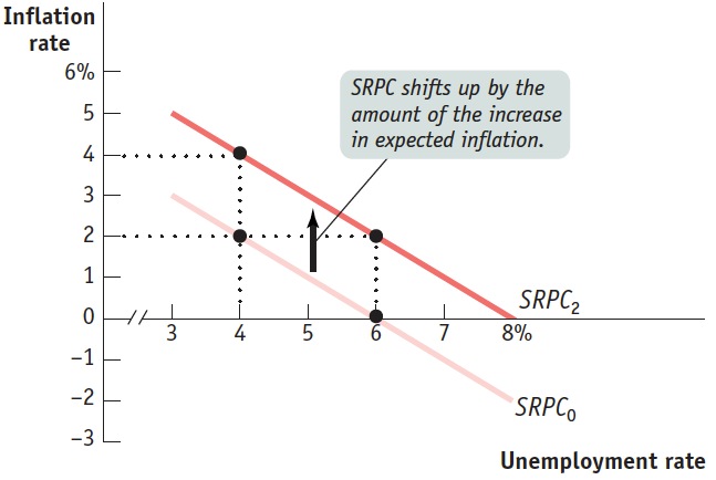
Figure 34.5: Expected Inflation and the Short-Run Phillips CurveAn increase in expected inflation shifts the short-run Phillips curve up. SRPC0 is the initial short-run Phillips curve with an expected inflation rate of 0%; SRPC2 is the short-run Phillips curve with an expected inflation rate of 2%. Each additional percentage point of expected inflation raises the actual inflation rate at any given unemployment rate by 1 percentage point.
AP® Exam Tip
Inflationary expectations shift the short-run AS curve as well as the short-run Phillips curve.
Alternatively, suppose the expected rate of inflation is 2%. In that case, employers and workers will build this expectation into wages and prices: at any given unemployment rate, the actual inflation rate will be 2 percentage points higher than it would be if people expected 0% inflation. SRPC2, which shows the Phillips curve when the expected inflation rate is 2%, is SRPC0 shifted upward by 2 percentage points at every level of unemployment. According to SRPC2, the actual inflation rate will be 2% if the unemployment rate is 6%; it will be 4% if the unemployment rate is 4%.
Page 332
From the Scary Seventies to the Nifty Nineties
From the Scary Seventies to the Nifty Nineties
Figure 34.1 showed that the American experience during the 1950s and 1960s supported the belief in the existence of a short-run Phillips curve for the U.S. economy, with a short-run trade-off between unemployment and inflation.
After 1969, however, that relationship appeared to fall apart according to the data. The figure here plots the course of U.S. unemployment and inflation rates from 1961 to 1990. As you can see, the course looks more like a tangled piece of yarn than like a smooth curve.
Through much of the 1970s and early 1980s, the economy suffered from a combination of above-average unemployment rates coupled with inflation rates unprecedented in modern American history. This condition came to be known as stagflation—for stagnation combined with high inflation. In the late 1990s, by contrast, the economy was experiencing a blissful combination of low unemployment and low inflation. What explains these developments?
Part of the answer can be attributed to a series of negative supply shocks that the U.S. economy suffered during the 1970s. The price of oil, in particular, soared as wars and revolutions in the Middle East led to a reduction in oil supplies and as oil-exporting countries deliberately curbed production to drive up prices. Compounding the oil price shocks, there was also a slowdown in labor productivity growth. Both of these factors shifted the short-run Phillips curve upward. During the 1990s, by contrast, supply shocks were positive. Prices of oil and other raw materials were generally falling, and productivity growth accelerated. As a result, the short-run Phillips curve shifted downward.
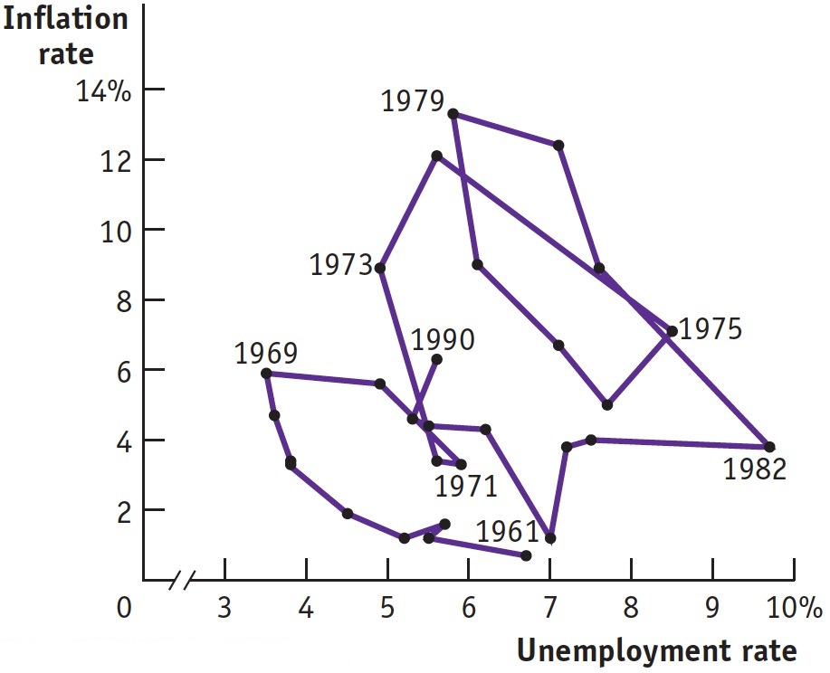
Source: Bureau of Labor Statistics.
Equally important, however, was the role of expected inflation. As mentioned earlier, inflation accelerated during the 1960s. During the 1970s, the public came to expect high inflation, and this also shifted the short-run Phillips curve up. It took a sustained and costly effort during the 1980s to get inflation back down. The result, however, was that expected inflation was very low by the late 1990s, allowing actual inflation to be low even with low rates of unemployment.
Page 333
What determines the expected rate of inflation? In general, people base their expectations about inflation on experience. If the inflation rate has hovered around 0% in the last few years, people will expect it to be around 0% in the near future. But if the inflation rate has averaged around 5% lately, people will expect inflation to be around 5% in the near future.
Since expected inflation is an important part of the modern discussion about the short-run Phillips curve, you might wonder why it was not in the original formulation of the Phillips curve. The answer lies in history. Think back to what we said about the early 1960s: at that time, people were accustomed to low inflation rates and reasonably expected that future inflation rates would also be low. It was only after 1965 that persistent inflation became a fact of life. So only then did it become clear that expected inflation would play an important role in price-setting.