Keynes’s ideas fundamentally changed the way economists think about business cycles. However, they did not go unquestioned. In the decades that followed the publication of The General Theory, Keynesian economics faced a series of challenges. As a result, the consensus of macroeconomists retreated somewhat from the strong version of Keynesianism that prevailed in the 1950s. In particular, economists became much more aware of the limits to macroeconomic policy activism.

Keynes’s The General Theory suggested that monetary policy wouldn’t be very effective in depression conditions. Many modern macroeconomists agree: earlier we introduced the concept of a liquidity trap, a situation in which monetary policy is ineffective because the interest rate is down against the zero bound. In the 1930s, when Keynes wrote, interest rates, in fact, were very close to 0%. (The term liquidity trap was first introduced by the British economist John Hicks in a 1937 paper, “Mr. Keynes and the Classics: A Suggested Interpretation,” that summarized Keynes’s ideas.)

But even when the era of near-0% interest rates came to an end after World War II, many economists continued to emphasize fiscal policy and downplay the usefulness of monetary policy. Eventually, however, macroeconomists reassessed the importance of monetary policy. A key milestone in this reassessment was the 1963 publication of A Monetary History of the United States, 1867–1960 by Milton Friedman, of the University of Chicago, and Anna Schwartz, of the National Bureau of Economic Research. Friedman and Schwartz showed that business cycles had historically been associated with fluctuations in the money supply. In particular, the money supply fell sharply during the onset of the Great Depression. Friedman and Schwartz persuaded many, though not all, economists that the Great Depression could have been avoided if the Federal Reserve had acted to prevent that monetary contraction. They persuaded most economists that monetary policy should play a key role in economic management.

The revival of interest in monetary policy was significant because it suggested that the burden of managing the economy could be shifted away from fiscal policy—meaning that economic management could largely be taken out of the hands of politicians. Fiscal policy, which must involve changing tax rates or government spending, necessitates political choices. If the government tries to stimulate the economy by cutting taxes, it must decide whose taxes will be cut. If it tries to stimulate the economy with government spending, it must decide what to spend the money on.

346

Monetary policy, by contrast, does not involve such choices: when the central bank cuts interest rates to fight a recession, it cuts everyone’s interest rate at the same time. So a shift from relying on fiscal policy to relying on monetary policy makes macroeconomics a more technical, less political issue. In fact, monetary policy in most major economies is set by an independent central bank that is insulated from the political process.

After the publication of A Monetary History, Milton Friedman led a movement, called monetarism, that sought to eliminate macroeconomic policy activism while maintaining the importance of monetary policy. Monetarism asserted that GDP will grow steadily if the money supply grows steadily. The monetarist policy prescription was to have the central bank target a constant rate of growth of the money supply, such as 3% per year, and maintain that target regardless of any fluctuations in the economy.

It’s important to realize that monetarism retained many Keynesian ideas. Like Keynes, Friedman asserted that the short run is important and that short-run changes in aggregate demand affect aggregate output as well as aggregate prices. Like Keynes, he argued that policy should have been much more expansionary during the Great Depression.

However, monetarists argued that most of the efforts of policy makers to smooth out the business cycle actually make things worse. We have already discussed concerns over the usefulness of discretionary fiscal policy—changes in taxes or government spending, or both—in response to the state of the economy. As we explained, government perceptions about the economy often lag behind reality, and there are further lags in changing fiscal policy and in its effects on the economy. As a result, discretionary fiscal policies intended to fight a recession often end up feeding a boom, and vice versa. According to monetarists, discretionary monetary policy, changes in the interest rate or the money supply by the central bank in order to stabilize the economy, faces the same problem of lags as fiscal policy, but to a lesser extent.

Friedman also argued that if the central bank followed his advice and refused to change the money supply in response to fluctuations in the economy, fiscal policy would be much less effective than Keynesians believed. Earlier we analyzed the phenomenon of crowding out, in which government deficits drive up interest rates and lead to reduced investment spending. Friedman and others pointed out that if the money supply is held fixed while the government pursues an expansionary fiscal policy, crowding out will limit the effect of the fiscal expansion on aggregate demand.

Figure 35.2 illustrates this argument. Panel (a) shows aggregate output and the aggregate price level. AD₁ is the initial aggregate demand curve and SRAS is the short-run aggregate supply curve. At the initial equilibrium, E₁, the level of aggregate output is Y₁ and the aggregate price level is P₁. Panel (b) shows the money market. MS is the money supply curve and MD₁ is the initial money demand curve, so the initial interest rate is r₁.

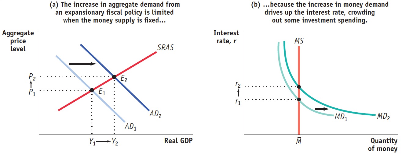
Now suppose the government increases purchases of goods and services. We know that this will shift the AD curve rightward, as illustrated by the shift from AD₁ to AD₂; that aggregate output will rise, from Y₁ to Y₂, and that the aggregate price level will rise, from P₁ to P₂. Both the rise in aggregate output and the rise in the aggregate price level, however, will increase the demand for money, shifting the money demand curve rightward from MD₁ to MD₂. This drives up the equilibrium interest rate to r₂. Friedman’s point was that this rise in the interest rate reduces investment spending, partially offsetting the initial rise in government spending. As a result, the rightward shift of the AD curve is smaller than multiplier analysis indicates. And Friedman argued that with a constant money supply, the multiplier is so small that there’s not much point in using fiscal policy.

But Friedman didn’t favor activist monetary policy either. He argued that the problem of time lags that limit the ability of discretionary fiscal policy to stabilize the economy also apply to discretionary monetary policy. Friedman’s solution was to put monetary policy on “autopilot.” The central bank, he argued, should follow a monetary policy rule, a formula that determines its actions and leaves it relatively little discretion. During the 1960s and 1970s, most monetarists favored a monetary policy rule of slow, steady growth in the money supply. Underlying this view was the Quantity Theory of Money, which relies on the concept of the velocity of money, the ratio of nominal GDP to the money supply. Velocity is a measure of the number of times the average dollar bill in the economy turns over per year between buyers and sellers (e.g., I tip the Starbucks barista a dollar, she uses it to buy lunch, and so on). This concept gives rise to the velocity equation:

347

(35-1) M × V = P × Y

Where M is the money supply, V is velocity, P is the aggregate price level, and Y is real GDP.

Monetarists believed, with considerable historical justification, that the velocity of money was stable in the short run and changed only slowly in the long run. As a result, they claimed, steady growth in the money supply by the central bank would ensure steady growth in spending, and therefore in GDP.

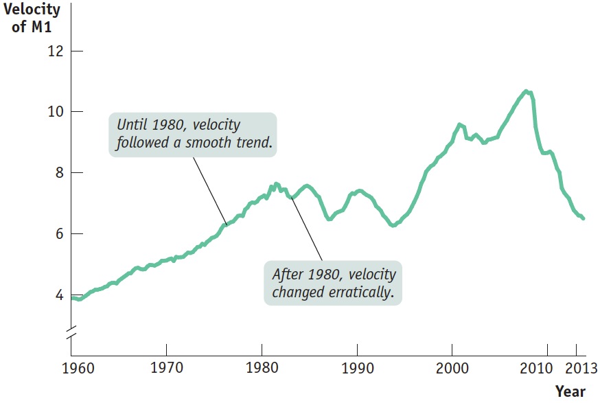
Monetarism strongly influenced actual monetary policy in the late 1970s and early 1980s. It quickly became clear, however, that steady growth in the money supply didn’t ensure steady growth in the economy: the velocity of money wasn’t stable enough for such a simple policy rule to work. Figure 35.3 shows how events eventually undermined the monetarists’ view. The figure shows the velocity of money, as measured by the ratio of nominal GDP to M1, from 1960 to the middle of 2013. As you can see, until 1980, velocity followed a fairly smooth, seemingly predictable trend. After the Fed began to adopt monetarist ideas in the late 1970s and early 1980s, however, the velocity of money began moving erratically—probably due to financial market innovations.

348

Traditional monetarists are hard to find among today’s macroeconomists. As we’ll see later, however, the concern that originally motivated the monetarists—that too much discretionary monetary policy can actually destabilize the economy—has become widely accepted.

At the same time that monetarists were challenging Keynesian views about how macroeconomic policy should be conducted, a somewhat broader group of economists was emphasizing the limits to what activist macroeconomic policy could achieve.

In the 1940s and 1950s, many Keynesian economists believed that expansionary fiscal policy could be used to achieve full employment on a permanent basis. In the 1960s, however, many economists realized that expansionary policies could cause problems with inflation, but they still believed policy makers could choose to trade off low unemployment for higher inflation even in the long run.

In 1968, however, Edmund Phelps of Columbia University and Milton Friedman, working independently, proposed the concept of the natural rate of unemployment. In Module 34 we saw that the natural rate of unemployment is also the nonaccelerating inflation rate of unemployment, or NAIRU. According to the natural rate hypothesis, because inflation is eventually embedded in expectations, to avoid accelerating inflation over time, the unemployment rate must be high enough that the actual inflation rate equals the expected rate of inflation. Attempts to keep the unemployment rate below the natural rate will lead to an ever-rising inflation rate.

The natural rate hypothesis limits the role of activist macroeconomic policy compared to earlier theories. Because the government can’t keep unemployment below the natural rate, its task is not to keep unemployment low but to keep it stable—to prevent large fluctuations in unemployment in either direction.

The Friedman–Phelps hypothesis made a strong prediction: that the apparent trade-off between unemployment and inflation would not survive an extended period of rising prices. Once inflation was embedded in the public’s expectations, inflation would continue even in the face of high unemployment. Sure enough, that’s exactly what happened in the 1970s. This accurate prediction was one of the triumphs of macroeconomic analysis, and it convinced the great majority of economists that the natural rate hypothesis was correct. In contrast to traditional monetarism, which declined in influence as more evidence accumulated, the natural rate hypothesis has become almost universally accepted among macroeconomists, with a few qualifications. (Some macroeconomists believe that at very low or negative rates of inflation the hypothesis doesn’t work.)

349

One final challenge to Keynesian economics focused not on the validity of the economic analysis but on its political consequences. A number of economists and political scientists pointed out that activist macroeconomic policy lends itself to political manipulation.

Statistical evidence suggests that election results tend to be determined by the state of the economy in the months just before the election. In the United States, if the economy is growing rapidly and the unemployment rate is falling in the six months or so before Election Day, the incumbent party tends to be re-elected even if the economy performed poorly in the preceding three years.

This creates an obvious temptation to abuse activist macroeconomic policy: pump up the economy in an election year, and pay the price in higher inflation and/or higher unemployment later. The result can be unnecessary instability in the economy, a political business cycle caused by the use of macroeconomic policy to serve political ends.

An often-cited example is the combination of expansionary fiscal and monetary policy that led to rapid growth in the U.S. economy just before the 1972 election and a sharp acceleration in inflation after the election. Kenneth Rogoff, a respected macroeconomist who served as chief economist at the International Monetary Fund, proclaimed Richard Nixon, the president at the time, “the all-time hero of political business cycles.”

One way to avoid a political business cycle is to place monetary policy in the hands of an independent central bank, insulated from political pressure. The political business cycle is also a reason to limit the use of discretionary fiscal policy to extreme circumstances.