Productivity is higher, other things equal, when workers are equipped with more physical capital, more human capital, better technology, or any combination of the three. But can we put numbers to these effects? To do this, economists make use of estimates of the aggregate production function, which shows how productivity depends on the quantities of physical capital per worker and human capital per worker as well as the state of technology. In general, all three factors tend to rise over time, as workers are equipped with more machinery, receive more education, and benefit from technological advances. What the aggregate production function does is allow economists to disentangle the effects of these three factors on overall productivity.

An example of an aggregate production function applied to real data comes from a comparative study of Chinese and Indian economic growth conducted by the economists Barry Bosworth and Susan Collins of the Brookings Institution. They used the following aggregate production function:

GDP per worker = T × (physical capital per worker)^0.4 × (human capital per worker)^0.6

where T represented an estimate of the level of technology and they assumed that each year of education raised workers’ human capital by 7%. Using this function, they tried to explain why China grew faster than India between 1978 and 2004. They found that about half the difference was due to China’s higher levels of investment spending, which raised its level of physical capital per worker faster than India’s. The other half was due to faster Chinese technological progress.

374

In analyzing historical economic growth, economists have discovered a crucial fact about the estimated aggregate production function: it exhibits diminishing returns to physical capital. That is, when the amount of human capital per worker and the state of technology are held fixed, each successive increase in the amount of physical capital per worker leads to a smaller increase in productivity. Table 38.1 gives a hypothetical example of how the level of physical capital per worker might affect the level of real GDP per worker, holding human capital per worker and the state of technology fixed. In this example, we measure the quantity of physical capital in terms of the dollars worth of investment.

As you can see from the table, there is a big payoff from the first $15,000 invested in physical capital: real GDP per worker rises by $30,000. The second $15,000 worth of physical capital also raises productivity, but not by as much: real GDP per worker goes up by only $15,000. The third $15,000 worth of physical capital raises real GDP per worker by only $10,000.

To see why the relationship between physical capital per worker and productivity exhibits diminishing returns, think about how having farm equipment affects the productivity of farm workers. A little bit of equipment makes a big difference: a worker equipped with a tractor can do much more than a worker without one. And, other things equal, a worker using more expensive equipment will be more productive: a worker with a $30,000 tractor will normally be able to cultivate more farmland in a given amount of time than a worker with a $15,000 tractor because the more expensive machine will be more powerful, perform more tasks, or both.

But will a worker with a $30,000 tractor, holding human capital and technology constant, be twice as productive as a worker with a $15,000 tractor? Probably not: there’s a huge difference between not having a tractor at all and having even an inexpensive tractor; there’s much less difference between having an inexpensive tractor and having a better tractor. And we can be sure that a worker with a $150,000 tractor won’t be 10 times as productive: a tractor can be improved only so much. Because the same is true of other kinds of equipment, the aggregate production function shows diminishing returns to physical capital.

Figure 38.1 is a graphical representation of the aggregate production function with diminishing returns to physical capital. As the productivity curve illustrates, more physical capital per worker leads to more output per worker. But each $30,000 increment in physical capital per worker adds less to productivity. By comparing points A, B, and C, you can also see that, as physical capital per worker rises, output per worker also rises—but at a diminishing rate. Going from point A to point B, representing a $30,000 increase in physical capital per worker, leads to an increase of $20,000 in real GDP per worker. Going from point B to point C, a second $30,000 increase in physical capital per worker, leads to an increase of only $10,000 in real GDP per worker.

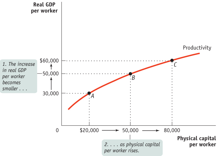
It’s important to realize that diminishing returns to physical capital is an “other things equal” phenomenon: additional amounts of physical capital are less productive when the amount of human capital per worker and the technology are held fixed. Diminishing returns may disappear if we increase the amount of human capital per worker, or improve the technology, or both when the amount of physical capital per worker is increased. For example, a worker with a $30,000 tractor who has also been trained in the most advanced cultivation techniques may in fact be more than twice as productive as a worker with only a $15,000 tractor and no additional human capital. But diminishing returns to any one input—regardless of whether it is physical capital, human capital, or labor—is a pervasive characteristic of production. Typical estimates suggest that, in practice, a 1% increase in the quantity of physical capital per worker increases output per worker by only one-third of 1%, or 0.33%.

375

In practice, all the factors contributing to higher productivity rise during the course of economic growth: both physical capital and human capital per worker increase, and technology advances as well. To disentangle the effects of these factors, economists use growth accounting to estimate the contribution of each major factor in the aggregate production function to economic growth. For example, suppose the following are true:

In that case, we would estimate that growing physical capital per worker is responsible for 1 percentage point (3% × 0.33) of productivity growth per year. A similar but more complex procedure is used to estimate the effects of growing human capital. The procedure is more complex because there aren’t simple dollar measures of the quantity of human capital.

Growth accounting allows us to calculate the effects of greater amounts of physical and human capital on economic growth. But how can we estimate the effects of technological progress? We can do so by estimating what is left over after the effects of physical and human capital have been taken into account. For example, let’s imagine that there was no increase in human capital per worker so that we can focus on changes in physical capital and in technology. In Figure 38.2, the lower curve shows the same hypothetical relationship between physical capital per worker and output per worker shown in Figure 38.1. Let’s assume that this was the relationship given the technology available in 1940. The upper curve also shows a relationship between physical capital per worker and productivity, but this time given the technology available in 2010. (We’ve chosen a 70-year stretch to allow us to use the Rule of 70.) The 2010 curve is shifted up compared to the 1940 curve because technologies developed over the previous 70 years make it possible to produce more output for a given amount of physical capital per worker than was possible with the technology available in 1940. (Note that the two curves are measured in constant dollars.)

376

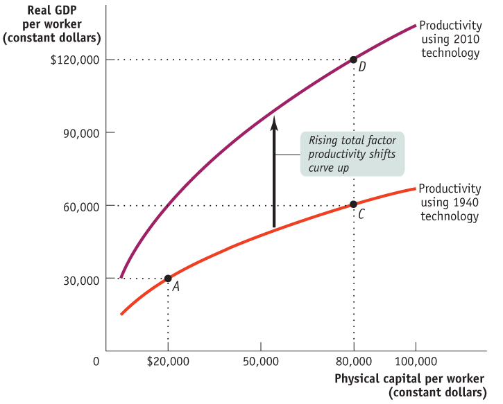
Let’s assume that between 1940 and 2010 the amount of physical capital per worker rose from $20,000 to $80,000. If this increase in physical capital per worker had taken place without any technological progress, the economy would have moved from A to C: output per worker would have risen, but only from $30,000 to $60,000, or 1% per year (using the Rule of 70 tells us that a 1% growth rate over 70 years doubles output). In fact, however, the economy moved from A to D: output rose from $30,000 to $120,000, or 2% per year. There was an increase in both physical capital per worker and technological progress, which shifted the aggregate production function.

In this case, 50% of the annual 2% increase in productivity—that is, 1% in annual productivity growth—is due to higher total factor productivity, the amount of output that can be produced with a given amount of factor inputs. So when total factor productivity increases, the economy can produce more output with the same quantity of physical capital, human capital, and labor.

377

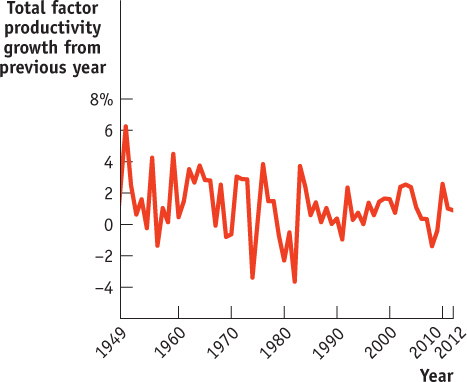
Most estimates find that increases in total factor productivity are central to a country’s economic growth. We believe that observed increases in total factor productivity in fact measure the economic effects of technological progress. All of this implies that technological change is crucial to economic growth. The Bureau of Labor Statistics estimates the growth rate of both labor productivity and total factor productivity for nonfarm business in the United States. According to the Bureau’s estimates, over the period from 1948 to 2010, American labor productivity rose 2.3% per year. Only 49% of that rise is explained by increases in physical and human capital per worker; the rest is explained by rising total factor productivity—that is, by technological progress.

In our discussion so far, we haven’t mentioned natural resources, which certainly have an effect on productivity. Other things equal, countries that are abundant in valuable natural resources, such as highly fertile land or rich mineral deposits, have higher real GDP per capita than less fortunate countries. The most obvious modern example is the Middle East, where enormous oil deposits have made a few sparsely populated countries very rich. For instance, Kuwait has about the same level of real GDP per capita as South Korea, but Kuwait’s wealth is based on oil, not manufacturing, the source of South Korea’s high output per worker.

But other things are often not equal. In the modern world, natural resources are a much less important determinant of productivity than human or physical capital for the great majority of countries. For example, some nations with very high real GDP per capita, such as Japan, have very few natural resources. Some resource-rich nations, such as Nigeria (which has sizable oil deposits), are very poor.

Historically, natural resources played a much more prominent role in determining productivity. In the nineteenth century, the countries with the highest real GDP per capita were those abundant in rich farmland and mineral deposits: the United States, Canada, Argentina, and Australia. As a consequence, natural resources figured prominently in the development of economic thought. In a famous book published in 1798, An Essay on the Principle of Population, the English economist Thomas Malthus made the fixed quantity of land in the world the basis of a pessimistic prediction about future productivity. As population grew, he pointed out, the amount of land per worker would decline. And, other things equal, this would cause productivity to fall. In fact, his view was that improvements in technology or increases in physical capital would lead only to temporary improvements in productivity because they would always be offset by the pressure of rising population and more workers on the supply of land. In the long run, he concluded, the great majority of people were condemned to living on the edge of starvation. Only then would death rates be high enough and birth rates low enough to prevent rapid population growth from outstripping productivity growth.

It hasn’t turned out that way, although many historians believe that Malthus’s prediction of falling or stagnant productivity was valid for much of human history. Population pressure probably did prevent large productivity increases until the eighteenth century. But in the time since Malthus wrote his book, any negative effects on productivity from population growth have been far outweighed by other, positive factors—advances in technology, increases in human and physical capital, and the opening up of enormous amounts of cultivatable land in the New World.

It remains true, however, that we live on a finite planet, with limited supplies of resources such as oil and limited ability to absorb environmental damage. We address the concerns these limitations pose for economic growth later in this section.

378