396

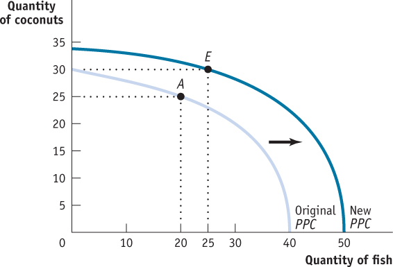
Recall from Section 1 that we defined the production possibilities curve as a graph that illustrates the trade-offs facing an economy that produces only two goods. In our example, we developed the production possibilities curve for Tom, a castaway facing a trade-off between producing fish and coconuts. Looking at Figure 40.2, we see that economic growth is shown as an outward shift of the production possibilities curve. Now let’s return to the production possibilities curve model and use a different example to illustrate how economic growth policies can lead to long-run economic growth.

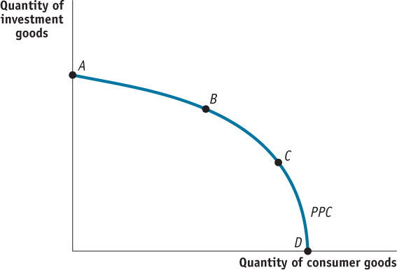
Figure 40.3 shows a hypothetical production possibilities curve for a fictional country we’ll call Kyland. In our previous production possibilities examples, the trade-off was between producing quantities of two different goods. In this example, our production possibilities curve illustrates Kyland’s trade-off between two different categories of goods. The production possibilities curve shows the alternative combinations of investment goods and consumer goods that Kyland can produce. The consumer goods category includes everything purchased for consumption by households, such as food, clothing, and sporting goods. Investment goods include all forms of physical capital, that is, goods that are used to produce other goods. Kyland’s production possibilities curve shows the trade-off between the production of consumer goods and the production of investment goods. Recall that the bowed-out shape of the production possibilities curve reflects increasing opportunity cost.

397

Kyland’s production possibilities curve shows all possible combinations of consumer and investment goods that can be produced with full and efficient use of all of Kyland’s resources. However, the production possibilities curve model does not tell us which of the possible points Kyland should select.

Figure 40.3 illustrates four points on Kyland’s production possibilities curve. At point A, Kyland is producing all investment goods and no consumer goods. Investment in physical capital, one of the economy’s factors of production, causes the production possibilities curve to shift outward. Choosing to produce at a point on the production possibilities curve that creates more capital for the economy will result in greater production possibilities in the future. Note that at point A, there are no consumer goods being produced, a situation which the economy cannot survive.

398

At point D, Kyland is producing all consumer goods and no investment goods. While this point provides goods and services for consumers in Kyland, it does not include the production of any physical capital. Over time, as an economy produces more goods and services, some of its capital is used up in that production. A loss in the value of physical capital due to wear, age, or obsolescence is called depreciation. If Kyland were to produce at point D year after year, it would soon find its stock of physical capital depreciating and its production possibilities curve would shift inward over time, indicating a decrease in production possibilities. Points B and C represent a mix of consumer and investment goods for the economy. While we can see that points A and D would not be acceptable choices over a long period of time, the choice between points B and C would depend on the values, politics, and other details related to the economy and people of Kyland. What we do know is that the choice made by Kyland each year will affect the position of the production possibilities curve in the future. An emphasis on the production of consumer goods will make consumers better off in the short run but will prevent the production possibilities curve from moving farther out in the future. An emphasis on investment goods will lead the production possibilities curve to shift out farther in the future but will decrease the quantity of consumer goods available in the short run.

So what does the production possibilities curve tell us about economic growth? Since long-run economic growth depends almost entirely on rising productivity, a country’s decision regarding investment in physical capital, human capital, and technology affects its long-run economic growth. Governments can promote long-run economic growth, shifting the country’s production possibilities curve outward over time, by investing in physical capital such as infrastructure. They can also encourage high rates of private investment in physical capital by promoting a well-functioning financial system, property rights, and political stability.