In our study of macroeconomics we have seen questions about the macroeconomy take many different forms. No matter what the specific question, most macroeconomic problems have the following components:

For example, you might be asked to consider the following scenario and answer the associated questions.

Assume the U.S. economy is currently operating at an aggregate output level above potential output. Draw a correctly labeled graph showing aggregate demand, short-run aggregate supply, long-run aggregate supply, equilibrium output, and the aggregate price level.

445

Now assume that the Federal Reserve conducts contractionary monetary policy. Identify the open-market operation the Fed would conduct, and draw a correctly labeled graph of the money market to show the effect of the monetary policy on the nominal interest rate.

Show and explain how the Fed’s actions will affect equilibrium in the aggregate demand and supply graph you drew previously. Indicate the new aggregate price level on your graph.

Assume Canada is the largest trading partner of the United States. Draw a correctly labeled graph of the foreign exchange market for the U.S. dollar showing how the change in the aggregate price level you indicate on your graph above will affect the foreign exchange market. What will happen to the value of the U.S. dollar relative to the Canadian dollar?

How will the Federal Reserve’s contractionary monetary policy affect the real interest rate in the United States in the long run? Explain.

Taken as a whole, this scenario and the associated questions can seem overwhelming. Let’s start by breaking down our analysis into four components.

Now we are ready to look at each of the steps and untangle this scenario.

Assume the U.S. economy is currently operating at an aggregate output level above potential output. Draw a correctly labeled graph showing aggregate demand, short-run aggregate supply, long-run aggregate supply, equilibrium output, and the aggregate price level.

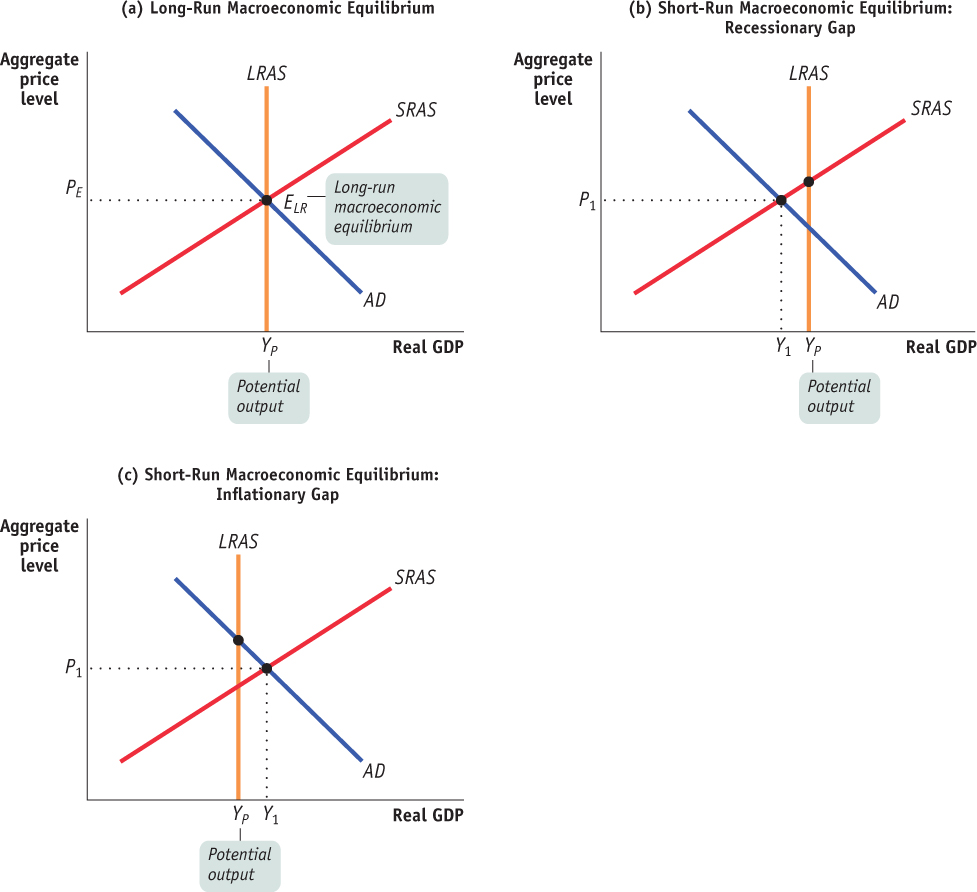
To analyze a situation, you have to know where to start. You will most often use the aggregate demand–aggregate supply model to evaluate macroeconomic scenarios. In this model, there are three possible starting points: long-run macroeconomic equilibrium, a recessionary gap, and an inflationary gap. This means that there are three possible “starting-point” graphs, as shown in Figure 45.1. The economy can be in long-run macroeconomic equilibrium with production at potential output as in panel (a); it can be in short-run macroeconomic equilibrium at an aggregate output level below potential output (creating a recessionary gap) as in panel (b); or it can be in short-run macroeconomic equilibrium at an aggregate output level above potential output (creating an inflationary gap) as in panel (c) and in our scenario.

Now assume that the Federal Reserve conducts contractionary monetary policy.

It is the events in a scenario that make it interesting. Perhaps a country goes into or recovers from a recession, inflation catches consumers off guard or becomes expected, consumers or businesses become more or less confident, holdings of money or wealth change, trading partners prosper or falter, or oil prices plummet or spike. The event can also be expansionary or contractionary monetary or fiscal policy. With the infinite number of possible changes in policy, politics, the economy, and markets around the world, don’t expect to analyze a familiar scenario on the exam.

While it’s impossible to foresee all of the scenarios you might encounter, we can group the determinants of change into a reasonably small set of major factors that influence macroeconomic models. Table 45.1 matches major factors with the curves they affect. With these influences in mind, it is relatively easy to proceed through a problem by identifying how the given events affect these factors. Most hypothetical scenarios involve changes in just one or two major factors. Although the real world is more complex, it is largely the same factors that change—there are just more of them changing at once.

Note: It is the real exchange rate (adjusted for international differences in aggregate price levels) that affects imports and exports.

446

As shown in Table 45.1, many curves are shifted by changes in only two or three major factors. Even for the aggregate demand curve, which has the largest number of associated factors, you can simplify the task further by asking yourself, “Does the event influence consumer spending, investment spending, government spending, or net exports?” If so, aggregate demand shifts. A shift of the long-run aggregate supply curve is caused only by events that affect labor productivity or the number of workers.

447

In the supply and demand model there are five major factors that shift the demand curve and five major factors that shift the supply curve. Most examples using this model will represent a change in one of these ten factors. The loanable funds market, money market, and foreign exchange market have their own clearly identified factors that affect supply or demand. With this information you can link specific events to relevant factors in the models to see what changes will occur. Remember that having correctly labeled axes on your graphs is crucial to a correct analysis.

Often, as in our scenario, the event is a policy response to an undesirable starting point such as a recessionary or inflationary gap. Expansionary policy is used to combat a recession, and contractionary policy is used to combat inflationary pressures. To begin analyzing a policy response, you need to fully understand how the Federal Reserve can implement each type of monetary policy (e.g., increase or decrease the money supply) and how that policy eventually affects the economy. You also need to understand how the government can implement expansionary or contractionary fiscal policy by raising or lowering taxes or government spending.

448

Show and explain how the Fed’s actions will affect equilibrium.

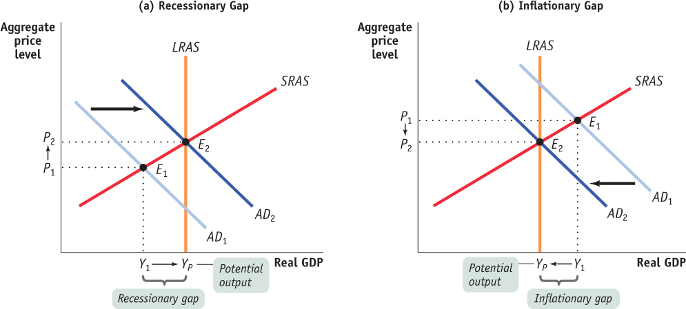
We have seen that events will create short-run effects in our models. In the short-run, fiscal and monetary policy both affect the economy by shifting the aggregate demand curve. As shown in panel (a) of Figure 45.2, expansionary policy shifts aggregate demand to the right, and as shown in panel (b), contractionary policy shifts aggregate demand to the left. To illustrate the effect of a policy response, shift the aggregate demand curve on your starting point graph and indicate the effects of the shift on the aggregate price level and aggregate output.

Assume Canada is the largest trading partner of the United States. What will happen to the value of the U.S. dollar relative to the Canadian dollar?

How will the Federal Reserve’s contractionary monetary policy affect the real interest rate in the United States in the long run? Explain.

Secondary Effects In addition to the initial, short-run effects of any event, there will be secondary effects and the economy will move to its long-run equilibrium after the short-run effects run their course.

We have seen that negative or positive demand shocks (including those created by inappropriate monetary or fiscal policy) move the economy away from long-run macroeconomic equilibrium. As explained in Module 18, in the absence of policy responses, such events will eventually be offset through changes in short-run aggregate supply resulting from changes in nominal wage rates. This will move the economy back to long-run macroeconomic equilibrium.

449

If the short-run effects of an action result in changes in the aggregate price level or real interest rate, there will also be secondary effects throughout the open economy. International capital flows and international trade will be affected as a result of the initial effects experienced in the economy. A price level decrease, as in our scenario, will encourage exports and discourage imports, causing an appreciation in the domestic currency on the foreign exchange market. A change in the interest rate affects aggregate demand through changes in investment spending and consumer spending. Interest rate changes also affect aggregate demand through changes in imports or exports caused by currency appreciation and depreciation. These secondary effects act to reinforce the effects of monetary policy.

Long-Run Effects While deviations from potential output are ironed out in the long run, other effects remain. For example, in the long run the use of fiscal policy affects the federal budget. Changes in taxes or government spending that lead to budget deficits (and increased federal debt) can “crowd out” private investment spending in the long run. The government’s increased demand for loanable funds drives up the interest rate, decreases investment spending, and partially offsets the initial increase in aggregate demand. Of course, the deficit could be addressed by printing money, but that would lead to problems with inflation in the long run.

We know that in the long run, monetary policy affects only the aggregate price level, not real GDP. Because money is neutral, changes in the money supply have no effect on the real economy. The aggregate price level and nominal values will be affected by the same proportion, leaving real values (including the real interest rate as mentioned in our scenario) unchanged.