Defining and Measuring Elasticity
As we saw in Section 1, dependent variables respond to changes in independent variables. For example, if two variables are negatively related and the independent variable increases, the dependent variable will respond by decreasing. But often the important question is not whether the variables are negatively or positively related, but how responsive the dependent variable is to changes in the independent variable (that is, by how much will the dependent variable change?). If price increases, we know that quantity demanded will decrease (that is the law of demand). The question in this context is by how much will quantity demanded decrease if price goes up?
AP® Exam Tip
Elasticity often appears on the AP® exam. Make sure you are able to calculate and interpret elasticity information.
Economists use the concept of elasticity to measure the responsiveness of one variable to changes in another. For example, price elasticity of demand measures the responsiveness of quantity demanded to changes in price—
Think back to the opening example of the flu shot panic. In order for Flunomics, a hypothetical flu vaccine distributor, to know whether it could raise its revenue by significantly raising the price of its flu vaccine, it would have to know whether the price increase would decrease the quantity demanded by a lot or a little. That is, it would have to know the price elasticity of demand for flu vaccinations.
Calculating the Price Elasticity of Demand
Figure 46.1 shows a hypothetical demand curve for flu vaccinations. At a price of $20 per vaccination, consumers would demand 10 million vaccinations per year (point A); at a price of $21, the quantity demanded would fall to 9.9 million vaccinations per year (point B).
| Figure 46.1 | The Demand for Vaccinations |
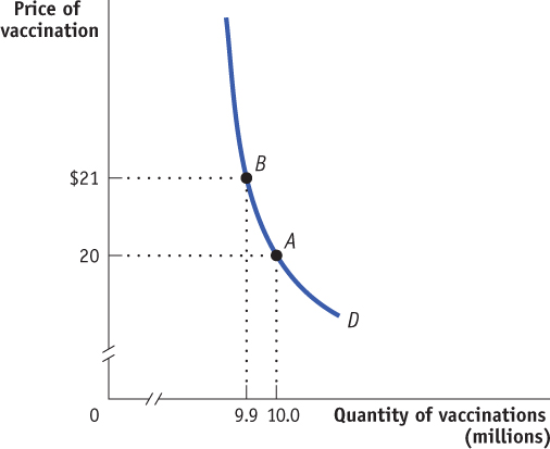
The price elasticity of demand is the ratio of the percent change in the quantity demanded to the percent change in the price as we move along the demand curve (dropping the minus sign).
Figure 46.1, then, tells us the change in the quantity demanded for a particular change in the price. But how can we turn this into a measure of price responsiveness? The answer is to calculate the price elasticity of demand. The price elasticity of demand compares the percent change in quantity demanded to the percent change in price as we move along the demand curve. As we’ll see later, economists use percent changes to get a measure that doesn’t depend on the units involved (say, a child-
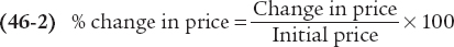
To calculate the price elasticity of demand, we first calculate the percent change in the quantity demanded and the corresponding percent change in the price as we move along the demand curve. These are defined as follows:

and
In Figure 46.1, we see that when the price rises from $20 to $21, the quantity demanded falls from 10 million to 9.9 million vaccinations, yielding a change in the quantity demanded of 0.1 million vaccinations. So the percent change in the quantity demanded is

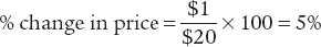
The initial price is $20 and the change in the price is $1, so the percent change in the price is
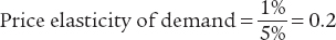
To calculate the price elasticity of demand, we find the ratio of the percent change in the quantity demanded to the percent change in the price:

In Figure 46.1, the price elasticity of demand is therefore
AP® Exam Tip
Be sure to use absolute values when computing the price elasticity of demand.
The law of demand says that demand curves slope downward, so price and quantity demanded always move in opposite directions. In other words, a positive percent change in price (a rise in price) leads to a negative percent change in the quantity demanded; a negative percent change in price (a fall in price) leads to a positive percent change in the quantity demanded. This means that the price elasticity of demand, in strictly mathematical terms, is a negative number. However, it is inconvenient to repeatedly write a minus sign. So when economists talk about the price elasticity of demand, they usually drop the minus sign and report the absolute value of the price elasticity of demand. In this case, for example, economists would usually say “the price elasticity of demand is 0.2,” taking it for granted that you understand they mean minus 0.2. We follow this convention here.
The larger the price elasticity of demand, the more responsive the quantity demanded is to the price. When the price elasticity of demand is large—
As we’ll see shortly, a price elasticity of 0.2 indicates a small response of quantity demanded to price. That is, the quantity demanded will fall by a relatively small amount when price rises. This is what economists call inelastic demand. And in the next module we’ll see why inelastic demand was exactly what Flunomics needed for its strategy to increase revenue by raising the price of its flu vaccines.
An Alternative Way to Calculate Elasticities: The Midpoint Method
We’ve seen that price elasticity of demand compares the percent change in quantity demanded with the percent change in price. When we look at some other elasticities, which we will do shortly, we’ll see why it is important to focus on percent changes. But at this point we need to discuss a technical issue that arises when you calculate percent changes in variables and how economists deal with it.
The best way to understand the issue is with a real example. Suppose you were trying to estimate the price elasticity of demand for gasoline by comparing gasoline prices and consumption in different countries. Because of high taxes, gasoline usually costs about three times as much per gallon in Europe as it does in the United States. So what is the percent difference between U.S. and European gas prices?
Well, it depends on which way you measure it. Because the price of gasoline in Europe is approximately three times higher than in the United States, it is 200 percent higher. Because the price of gasoline in the United States is one-
In our previous example, we found an elasticity of demand for vaccinations of 0.200 when considering a movement from point A to point B. However, when going from point B to point A, the same elasticity formula would indicate an elasticity of 0.212. This is a nuisance: we’d like to have an elasticity measure that doesn’t depend on the direction of change. A good way to avoid computing different elasticities for rising and falling prices is to use the midpoint method (sometimes called the arc method).
The midpoint method is a technique for calculating the percent change by dividing the change in a variable by the average, or midpoint, of the initial and final values of that variable.
The midpoint method replaces the usual definition of the percent change in a variable, X, with a slightly different definition:
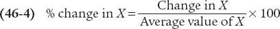
where the average value of X is defined as

AP® Exam Tip
The midpoint formula yields the same elasticity for a specified range regardless of the direction of the change in price.
When calculating the price elasticity of demand using the midpoint method, both the percent change in the price and the percent change in the quantity demanded are found using average values in this way. To see how this method works, suppose you have the following data for chocolate bars:
| Price | Quantity demanded | |
| Situation A | $0.90 | 1,100 |
| Situation B | $1.10 | 900 |
To calculate the percent change in quantity going from situation A to situation B, we compare the change in the quantity demanded—

In the same way, we calculate the percent change in price as

So in this case we would calculate the price elasticity of demand to be

again dropping the minus sign.
The important point is that we would get the same result, a price elasticity of demand of 1, whether we went up the demand curve from situation A to situation B or down from situation B to situation A.
To arrive at a more general formula for price elasticity of demand, suppose that we have data for two points on a demand curve. At point 1 the quantity demanded and the price are (Q1, P1); at point 2 they are (Q2, P2). Then the formula for calculating the price elasticity of demand is:
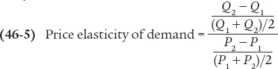
As before, when reporting a price elasticity of demand calculated by the midpoint method, we drop the minus sign and report the absolute value.
Estimating Elasticities
Estimating Elasticities
You might think it’s easy to estimate price elasticities of demand from real-
The most comprehensive effort to estimate price elasticities of demand was a mammoth study by the economists Hendrik S. Houthakker and Lester D. Taylor. Some of their results are summarized in Table 46.1. These estimates show a wide range of price elasticities. There are some goods, like eggs, for which demand hardly responds at all to changes in the price; there are other goods, most notably foreign travel, for which the quantity demanded is very sensitive to the price.
Table 46.1Some Estimated Price Elasticities of Demand
| Good | Price elasticity of demand |
| Inelastic demand | |
| Eggs | 0.1 |
| Beef | 0.4 |
| Stationery | 0.5 |
| Gasoline | 0.5 |
| Elastic demand | |
| Housing | 1.2 |
| Restaurant meals | 2.3 |
| Airline travel | 2.4 |
| Foreign travel | 4.1 |
|
Source: Hendrick S. Houthakker and Lester D. Taylor, Consumer Demand in the United States, 1929– |
|
Notice that Table 46.1 is divided into two parts: inelastic and elastic demand. We’ll explain the significance of that division in the next section.