Consumer Surplus and the Demand Curve
First-year college students are often surprised by the prices of the textbooks required for their classes. The College Board estimates that in 2013–2014 students at public four-year schools, on average, spent $1,207 for books and supplies. But at the end of the semester, students might again be surprised to find out that they can sell back at least some of the textbooks they used for the semester for a percentage of the purchase price (offsetting some of the cost of textbooks). The ability to purchase used textbooks at the start of the semester and to sell back used textbooks at the end of the semester is beneficial to students on a budget. In fact, the market for used textbooks is a big business in terms of dollars and cents—approximately $1.5 billion in 2011–2012. This market provides a convenient starting point for us to develop the concepts of consumer and producer surplus. We’ll use the concepts of consumer and producer surplus to understand exactly how buyers and sellers benefit from a competitive market and how big those benefits are. In addition, these concepts assist in the analysis of what happens when competitive markets don’t work well or there is interference in the market.
Let’s begin by looking at the market for used textbooks, starting with the buyers. The key point, as we’ll see in a minute, is that the demand curve is derived from their tastes or preferences—and that those same preferences also determine how much they gain from the opportunity to buy used books.
Willingness to Pay and the Demand Curve
A consumer’s willingness to pay for a good is the maximum price at which he or she would buy that good.
A used book is not as good as a new book—it will be battered and coffee-stained, may include someone else’s highlighting, and may not be completely up to date. How much this bothers you depends on your preferences. Some potential buyers would prefer to buy the used book even if it is only slightly cheaper than a new one, while others would buy the used book only if it is considerably cheaper. Let’s define a potential buyer’s willingness to pay as the maximum price at which he or she would buy a good, in this case a used textbook. An individual won’t buy the good if it costs more than this amount but is eager to do so if it costs less. If the price is just equal to an individual’s willingness to pay, he or she is indifferent between buying and not buying. For the sake of simplicity, we’ll assume that the individual buys the good in this case.
The table in Figure 49.1 shows five potential buyers of a used book that costs $100 new, listed in order of their willingness to pay. At one extreme is Aleisha, who will buy a second-hand book even if the price is as high as $59. Brad is less willing to have a used book and will buy one only if the price is $45 or less. Claudia is willing to pay only $35 and Darren, only $25. Edwina, who really doesn’t like the idea of a used book, will buy one only if it costs no more than $10.
| Figure 49.1 | The Demand Curve for Used Textbooks |
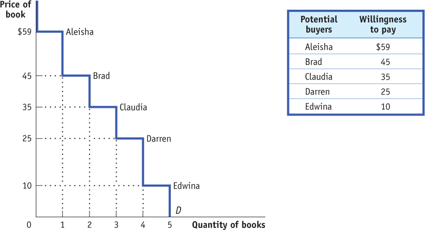
Figure 49.1: The Demand Curve for Used TextbooksWith only five potential consumers in this market, the demand curve is step-shaped. Each step represents one consumer, and its height indicates that consumer’s willingness to pay—the maximum price at which each will buy a used textbook—as indicated in the table. Aleisha has the highest willingness to pay at $59, Brad has the next highest at $45, and so on down to Edwina with the lowest willingness to pay at $10. At a price of $59, the quantity demanded is one (by Aleisha); at a price of $45, the quantity demanded is two (by Aleisha and Brad); and so on until you reach a price of $10, at which all five students are willing to purchase a book.
How many of these five students will actually buy a used book? It depends on the price. If the price of a used book is $55, only Aleisha buys one; if the price is $40, Aleisha and Brad both buy used books, and so on. So the information in the table can be used to construct the demand schedule for used textbooks.
We can use this demand schedule to derive the market demand curve shown in Figure 49.1. Because we are considering only a small number of consumers, this curve doesn’t look like the smooth demand curves we have seen previously, for markets that contained hundreds or thousands of consumers. This demand curve is step-shaped, with alternating horizontal and vertical segments. Each horizontal segment—each step—corresponds to one potential buyer’s willingness to pay. However, we’ll see shortly that for the analysis of consumer surplus it doesn’t matter whether the demand curve is step-shaped, as in this figure, or whether there are many consumers, making the curve smooth.
Page 487
Willingness to Pay and Consumer Surplus
Suppose that the campus bookstore makes used textbooks available at a price of $30. In that case Aleisha, Brad, and Claudia will buy books. Do they gain from their purchases, and if so, how much?
The answer, shown in Table 49.1, is that each student who purchases a book does achieve a net gain, but that the amount of the gain differs among students. Aleisha would have been willing to pay $59, so her net gain is $59 – $30 = $29. Brad would have been willing to pay $45, so his net gain is $45 – $30 = $15. Claudia would have been willing to pay $35, so her net gain is $35 – $30 = $5. Darren and Edwina, however, won’t be willing to buy a used book at a price of $30, so they neither gain nor lose.
Table 49.1Consumer Surplus When the Price of a Used Textbook Is $30
| Potential buyer |
Willingness to pay |
Price paid |
Individual consumer surplus = Willingness to pay − Price paid |
| Aleisha |
$59 |
$30 |
$29 |
| Brad |
45 |
30 |
15 |
| Claudia |
35 |
30 |
5 |
| Darren |
25 |
– |
– |
| Edwina |
10 |
– |
– |
| All buyers |
|
|
Total consumer surplus = $49 |
Table 49.1: Table 49.1 Consumer Surplus When the Price of a Used Textbook Is \$30
Individual consumer surplus is the net gain to an individual buyer from the purchase of a good. It is equal to the difference between the buyer’s willingness to pay and the price paid.
Total consumer surplus is the sum of the individual consumer surpluses of all the buyers of a good in a market.
The term consumer surplus is often used to refer to both individual and total consumer surplus.
The net gain that a buyer achieves from the purchase of a good is called that buyer’s individual consumer surplus. What we learn from this example is that whenever a buyer pays a price less than his or her willingness to pay, the buyer achieves some individual consumer surplus.
The sum of the individual consumer surpluses achieved by all the buyers of a good is known as the total consumer surplus achieved in the market. In Table 49.1, the total consumer surplus is the sum of the individual consumer surpluses achieved by Aleisha, Brad, and Claudia: $29 + $15 + $5 = $49.
Page 488
Economists often use the term consumer surplus to refer to both individual and total consumer surplus. We will follow this practice; it will always be clear in context whether we are referring to the consumer surplus achieved by an individual or by all buyers.
Total consumer surplus can be represented graphically. Figure 49.2 reproduces the demand curve from Figure 49.1. Each step in that demand curve is one book wide and represents one consumer. For example, the height of Aleisha’s step is $59, her willingness to pay. This step forms the top of a rectangle, with $30—the price she actually pays for a book—forming the bottom. The area of Aleisha’s rectangle, ($59 –$30) × 1 = $29, is her consumer surplus from purchasing one book at $30. So the individual consumer surplus Aleisha gains is the area of the dark blue rectangle shown in Figure 49.2.
| Figure 49.2 | Consumer Surplus in the Used-Textbook Market |
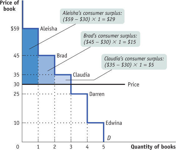
Figure 49.2: Consumer Surplus in the Used-Textbook MarketAt a price of $30, Aleisha, Brad, and Claudia each buy a book but Darren and Edwina do not. Aleisha, Brad, and Claudia get individual consumer surpluses equal to the difference between their willingness to pay and the price, illustrated by the areas of the shaded rectangles. Both Darren and Edwina have a willingness to pay less than $30, so they are unwilling to buy a book in this market; they receive zero consumer surplus. The total consumer surplus is given by the entire shaded area—the sum of the individual consumer surpluses of Aleisha, Brad, and Claudia—equal to $29 + $15 + $5 = $49.
In addition to Aleisha, Brad and Claudia will also each buy a book when the price is $30. Like Aleisha, they benefit from their purchases, though not as much, because they each have a lower willingness to pay. Figure 49.2 also shows the consumer surplus gained by Brad and Claudia; again, this can be measured by the areas of the appropriate rectangles. Darren and Edwina, because they do not buy books at a price of $30, receive no consumer surplus.
Page 489
AP® Exam Tip
You may be asked to calculate the size of the area that represents consumer surplus, which is bounded by the demand curve, the price line, and the vertical axis. Remember: the area of a triangle is ½ the base times the height.
The total consumer surplus achieved in this market is just the sum of the individual consumer surpluses received by Aleisha, Brad, and Claudia. So total consumer surplus is equal to the combined area of the three rectangles—the entire shaded area in Figure 49.2. Another way to say this is that total consumer surplus is equal to the area below the demand curve but above the price.
This is worth repeating as a general principle: The total consumer surplus generated by purchases of a good at a given price is equal to the area below the demand curve but above that price. The same principle applies regardless of the number of consumers.
When we consider large markets, this graphical representation becomes particularly helpful. Consider, for example, the sales of personal computers to millions of potential buyers. Each potential buyer has a maximum price that he or she is willing to pay. With so many potential buyers, the demand curve will be smooth, like the one shown in Figure 49.3.
| Figure 49.3 | Consumer Surplus |
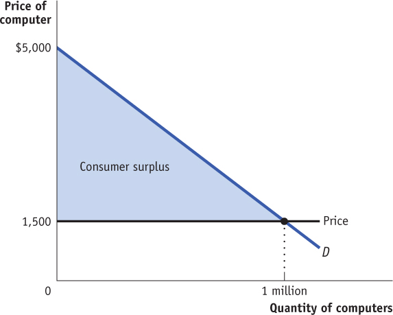
Figure 49.3: Consumer SurplusThe demand curve for computers is smooth because there are many potential buyers. At a price of $1,500, 1 million computers are demanded. The consumer surplus at this price is equal to the shaded area: the area below the demand curve but above the price. The area of a triangle is ½ × the base of the triangle × the height of the triangle. So the total consumer surplus in this case is ½ × 1 million × $3,500 = $1.75 billion. This is the total net gain to consumers generated from buying and consuming computers when the price is $1,500.
Suppose that at a price of $1,500, a total of 1 million computers are purchased. How much do consumers gain from being able to buy those 1 million computers? We could answer that question by calculating the individual consumer surplus of each buyer and then adding these numbers up to arrive at a total. But it is much easier just to look at Figure 49.3 and use the fact that total consumer surplus is equal to the shaded area below the demand curve but above the price. Recall that the area of a triangle is ½ × the base of the triangle × the height of the triangle. So the total consumer surplus in this case is ½ × 1 million × $3,500 = $1.75 billion.
How Changing Prices Affect Consumer Surplus
It is often important to know how price changes affect consumer surplus. For example, we may want to know the harm to consumers from a frost in Florida that drives up the prices of oranges, or consumers’ gain from the introduction of fish farming that makes salmon steaks less expensive. The same approach we have used to derive consumer surplus can be used to answer questions about how changes in prices affect consumers.

iStockphoto
Let’s return to the example of the market for used textbooks. Suppose that the bookstore decided to sell used textbooks for $20 instead of $30. By how much would this fall in price increase consumer surplus?
Page 490
The answer is illustrated in Figure 49.4. As shown in the figure, there are two parts to the increase in consumer surplus. The first part, shaded dark blue, is the gain of those who would have bought books even at the higher price of $30. Each of the students who would have bought books at $30—Aleisha, Brad, and Claudia—now pays $10 less, and therefore each gains $10 in consumer surplus from the fall in price to $20. So the dark blue area represents the $10 × 3 = $30 increase in consumer surplus to those three buyers. The second part, shaded light blue, is the gain to those who would not have bought a book at $30 but are willing to pay more than $20. In this case that gain goes to Darren, who would not have bought a book at $30 but does buy one at $20. He gains $5—the difference between his willingness to pay of $25 and the new price of $20. So the light blue area represents a further $5 gain in consumer surplus. The total increase in consumer surplus is the sum of the shaded areas, $35. Likewise, a rise in price from $20 to $30 would decrease consumer surplus by an amount equal to the sum of the shaded areas.
| Figure 49.4 | Consumer Surplus and a Fall in the Price of Used Textbooks |
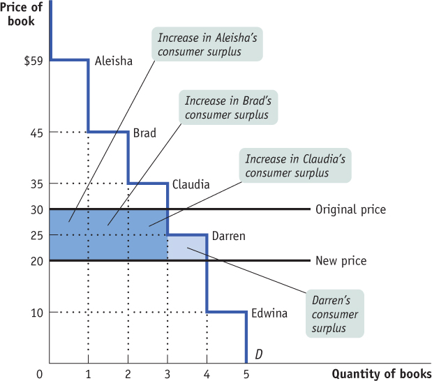
Figure 49.4: Consumer Surplus and a Fall in the Price of Used TextbooksThere are two parts to the increase in consumer surplus generated by a fall in price from $30 to $20. The first is given by the dark blue rectangle: each person who would have bought at the original price of $30—Aleisha, Brad, and Claudia—receives an increase in consumer surplus equal to the total reduction in price, $10. So the area of the dark blue rectangle corresponds to an amount equal to 3 × $10 = $30. The second part is given by the light blue area: the increase in consumer surplus for those who would not have bought at the original price of $30 but who buy at the new price of $20—namely, Darren. Darren’s willingness to pay is $25, so he now receives consumer surplus of $5. The total increase in consumer surplus is 3 × $10 + $5 = $35, represented by the sum of the shaded areas. Likewise, a rise in price from $20 to $30 would decrease consumer surplus by an amount equal to the sum of the shaded areas.
Figure 49.4 illustrates that when the price of a good falls, the area under the demand curve but above the price—the total consumer surplus—increases. Figure 49.5 shows the same result for the case of a smooth demand curve for personal computers. Here we assume that the price of computers falls from $4,300 to $1,500, leading to an increase in the quantity demanded from 200,000 to 1 million units. As in the used-textbook example, we divide the gain in consumer surplus into two parts. The dark blue rectangle in Figure 49.5 corresponds to the dark blue area in Figure 49.4: it is the gain to the 200,000 people who would have bought computers even at the higher price of $4,300. As a result of the price reduction, each receives additional surplus of $2,800, so the area of the dark blue rectangle is 200,000 × $2,800 = $560 million. The light blue triangle in Figure 49.5 corresponds to the light blue area in Figure 49.4: it is the gain to people who would not have bought the good at the higher price but are willing to do so at a price of $1,500. For example, the light blue triangle includes the gain to someone who would have been willing to pay $2,000 for a computer and therefore gains $500 in consumer surplus when it is possible to buy a computer for only $1,500. The area of the light blue triangle is ½ × 800,000 × $2,800 = $1.12 billion. As before, the total gain in consumer surplus is the sum of the shaded areas, the increase in the area under the demand curve but above the price: $560 million + $1.12 billion = $1.68 billion.
Page 491
| Figure 49.5 | A Fall in the Price Increases Consumer Surplus |
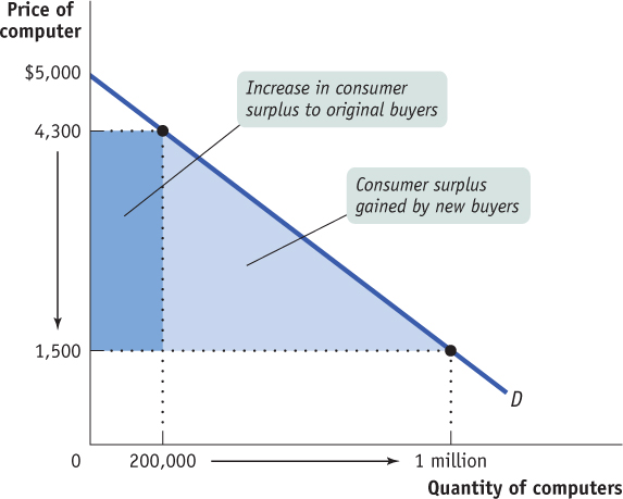
Figure 49.5: A Fall in the Price Increases Consumer SurplusA fall in the price of a computer from $4,300 to $1,500 leads to an increase in the quantity demanded and an increase in consumer surplus. The change in total consumer surplus is given by the sum of the shaded areas: the total area below the demand curve and between the old and new prices. Here, the dark blue area represents the increase in consumer surplus for the 200,000 consumers who would have bought a computer at the original price of $4,300; they each receive an increase in consumer surplus of $2,800. The light blue area represents the increase in consumer surplus for those willing to buy at a price equal to or greater than $1,500 but less than $4,300. Similarly, a rise in the price of a computer from $1,500 to $4,300 generates a decrease in consumer surplus equal to the sum of the two shaded areas.
A Matter of Life and Death
A Matter of Life and Death
Each year about 4,000 people in the United States die while waiting for a kidney transplant. In 2014, some 99,200 were on the waiting list. Since the number of those in need of a kidney far exceeds availability, what is the best way to allocate available organs? A market isn’t feasible. For understandable reasons, the sale of human body parts is illegal in this country. So the task of establishing a protocol for these situations has fallen to the nonprofit group United Network for Organ Sharing (UNOS).
Under current UNOS guidelines, a donated kidney goes to the person who has been waiting the longest. According to this system, an available kidney would go to a 75-year-old who has been waiting for 2 years instead of to a 25-year-old who has been waiting 6 months, even though the 25-year-old will likely live longer and benefit from the transplanted organ for a longer period of time.
To address this issue, the UNOS Kidney Transplantation Committee has proposed a new set of guidelines based on a concept it calls “net benefit.” According to these new guidelines, kidneys would be allocated on the basis of who will receive the greatest net benefit, where net benefit is measured as the expected increase in lifespan from the transplant. And age is by far the biggest predictor of how long someone will live after a transplant. For example, a typical 25-year-old diabetic will gain an extra 8.7 years of life from a transplant, but a typical 55-year-old diabetic will gain only 3.6 extra years.
Under the current system, based on waiting times, transplants lead to about 44,000 extra years of life for recipients; under the proposed system, that number would jump to 55,000 extra years. The share of kidneys going to those in their 20s would triple; the share going to those 60 and older would be halved.
What does this have to do with consumer surplus? As you may have guessed, the UNOS concept of “net benefit” is a lot like individual consumer surplus—the individual consumer surplus generated from getting a new kidney. In essence, the proposed system would allocate donated kidneys according to who gets the greatest individual consumer surplus. In terms of results, then, its proposed “net benefit” system would operate a lot like a competitive market.

Ray Roper/Getty Images
Page 492
What would happen if the price of a good were to rise instead of fall? We would do the same analysis in reverse. Suppose, for example, that for some reason the price of computers rises from $1,500 to $4,300. This would lead to a fall in consumer surplus equal to the sum of the shaded areas in Figure 49.5. This loss consists of two parts. The dark blue rectangle represents the loss to consumers who would still buy a computer, even at a price of $4,300. The light blue triangle represents the loss to consumers who decide not to buy a computer at the higher price.