In the previous module we learned about different types of profit, how to calculate profit, and how firms can use profit calculations to make decisions—for instance to determine whether to continue using resources for the same activity or not. In this module we ask the question: what quantity of output would maximize the producer’s profit? First we will find the profit-maximizing quantity by calculating the total profit at each quantity for comparison. Then we will use marginal analysis to determine the optimal output rule, which turns out to be simple: as our discussion of marginal analysis in Module 1 suggested, a producer should produce up until marginal benefit equals marginal cost.

Consider Jennifer and Jason, who run an organic tomato farm. Suppose that the market price of organic tomatoes is $18 per bushel and that Jennifer and Jason can sell as many as they would like at that price. Then we can use the data in Table 53.1 to find their profit-maximizing level of output.

The first column shows the quantity of output in bushels, and the second column shows Jennifer and Jason’s total revenue from their output: the market value of their output. Total revenue, TR, is equal to the market price multiplied by the quantity of output:

(53-1) TR = P × Q

In this example, total revenue is equal to $18 per bushel times the quantity of output in bushels.

The third column of Table 53.1 shows Jennifer and Jason’s total cost, TC. Even if they don’t grow any tomatoes, Jennifer and Jason must pay $14 to rent the land for their farm. As the quantity of tomatoes increases, so does the total cost of seeds, fertilizer, labor, and other inputs. You will learn more about firm costs in Module 55.

540

The fourth column shows their profit, equal to total revenue minus total cost:

(53-2) Profit = TR – TC

As indicated by the numbers in the table, profit is maximized at an output of five bushels, where profit is equal to $18. But we can gain more insight into the profit-maximizing choice of output by viewing it as a problem of marginal analysis, a task we’ll dive into next.

The principle of marginal analysis provides a clear message about when to stop doing anything: proceed until marginal benefit equals marginal cost. To apply this principle, consider the effect on a producer’s profit of increasing output by one unit. The marginal benefit of that unit is the additional revenue generated by selling it; this measure has a name—it is called the marginal revenue of that output. The general formula for marginal revenue is:

or

MR = ΔTR/ΔQ

In this equation, the Greek uppercase delta (the triangular symbol) represents the change in a variable.

The application of the principle of marginal analysis to the producer’s decision of how much to produce is called the optimal output rule, which states that profit is maximized by producing the quantity at which the marginal revenue of the last unit produced is equal to its marginal cost. As this rule suggests, we will see that Jennifer and Jason maximize their profit by equating marginal revenue and marginal cost.

Note that there may not be any particular quantity at which marginal revenue exactly equals marginal cost. In this case the producer should produce until one more unit would cause marginal benefit to fall below marginal cost. As a common simplification, we can think of marginal cost as rising steadily, rather than jumping from one level at one quantity to a different level at the next quantity. This ensures that marginal cost will equal marginal revenue at some quantity. We employ this simplified approach in what follows.

541

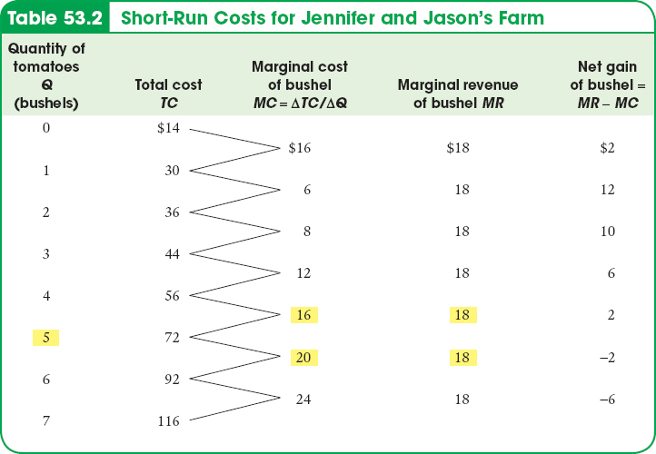
Consider Table 53.2, which provides cost and revenue data for Jennifer and Jason’s farm. The second column contains the farm’s total cost of output. The third column shows their marginal cost. Notice that, in this example, marginal cost initially falls as output rises but then begins to increase, so that the marginal cost curve has a “swoosh” shape. Later it will become clear that this shape has important implications for short-run production decisions.

The fourth column contains the farm’s marginal revenue, which has an important feature: Jennifer and Jason’s marginal revenue is assumed to be constant at $18 for every output level. The assumption holds true for a particular type of market—perfectly competitive markets—which we will study in Modules 58–60, but for now it is just to make the calculations easier. The fifth and final column shows the calculation of the net gain per bushel of tomatoes, which is equal to marginal revenue minus marginal cost. As you can see, it is positive for the first through fifth bushels: producing each of these bushels raises Jennifer and Jason’s profit. For the sixth and seventh bushels, however, net gain is negative: producing them would decrease, not increase, profit. (You can verify this by reexamining Table 53.1.) So five bushels are Jennifer and Jason’s profit-maximizing output; it is the level of output at which marginal cost is equal to the market price, $18.

Figure 53.1 shows that Jennifer and Jason’s profit-maximizing quantity of output is, indeed, the number of bushels at which the marginal cost of production is equal to marginal revenue (which is equivalent to price in perfectly competitive markets). The figure illustrates the marginal cost curve, MC, which shows the relationship between marginal cost and output. We plot the marginal cost of increasing output from one to two bushels halfway between one and two, and so on. The horizontal line at $18 is Jennifer and Jason’s marginal revenue curve, which shows the relationship between marginal revenue and output. Note that marginal revenue stays the same regardless of how much Jennifer and Jason sell because we have assumed marginal revenue is constant.

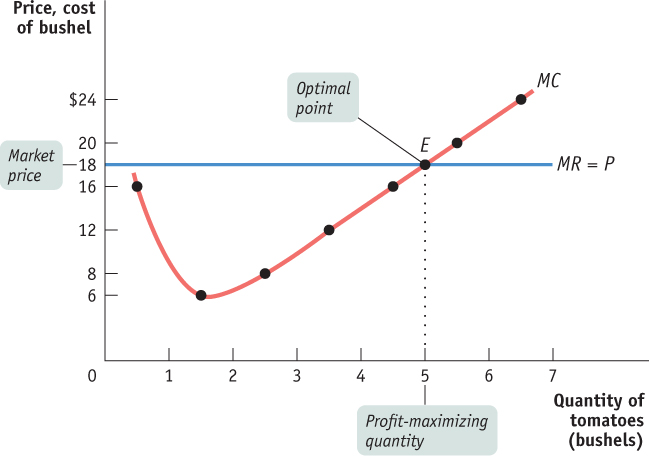
Does this mean that the firm’s production decision can be entirely summed up as “produce up to the point where the marginal cost of production is equal to the price”? No, not quite. Before applying the principle of marginal analysis to determine how much to produce, a potential producer must, as a first step, answer an “either–or” question: Should I produce at all? If the answer to that question is yes, the producer then proceeds to the second step—a “how much” decision: maximizing profit by choosing the quantity of output at which marginal cost is equal to price.

542

To understand why the first step in the production decision involves an “either–or” question, we need to ask how we determine whether it is profitable or unprofitable to produce at all.

Recall that a firm’s decision whether or not to stay in a given business in the long run depends on its economic profit—a measure based on the opportunity cost of resources used in the business. To put it a slightly different way: in the calculation of economic profit, a firm’s total cost incorporates the implicit cost—the benefits forgone in the next best use of the firm’s resources—as well as the explicit cost in the form of actual cash outlays. In contrast, accounting profit is profit calculated using only the explicit costs incurred by the firm. This means that economic profit incorporates the opportunity cost of resources owned by the firm and used in the production of output, while accounting profit does not. As in the example of Babette’s Cajun Café, a firm may make positive accounting profit while making zero or even negative economic profit. It’s important to understand clearly that a firm’s long-run decision to produce or not, to stay in business or to close down permanently, should be based on economic profit, not accounting profit.

So we will assume, as we always do, that the cost numbers given in Tables 53.1 and 53.2 include all costs, implicit as well as explicit, and that the profit numbers in Table 53.1 are economic profit. What determines whether Jennifer and Jason’s farm earns a profit or generates a loss? The answer is that whether or not it is profitable depends on the market price of tomatoes—specifically, whether selling the firm’s optimal quantity of output at the market price results in at least a normal profit.

In the next modules, we look in detail at the two components used to calculate profit: firm revenue (which is determined by the level of production) and firm cost.