MODULE 54: The Production Function

The Production Function

A production function is the relationship between the quantity of inputs a firm uses and the quantity of output it produces.

A firm produces goods or services for sale. To do this, it must transform inputs into output. The quantity of output a firm produces depends on the quantity of inputs; this relationship is known as the firm’s production function. As we’ll see, a firm’s production function underlies its cost curves. As a first step, let’s look at the characteristics of a hypothetical production function.

Inputs and Output

To understand the concept of a production function, let’s consider a farm that we assume, for the sake of simplicity, produces only one output, wheat, and uses only two inputs, land and labor. This particular farm is owned by a couple named George and Martha. They hire workers to do the actual physical labor on the farm. Moreover, we will assume that all potential workers are of the same quality—they are all equally knowledgeable and capable of performing farmwork.

A fixed input is an input whose quantity is fixed for a period of time and cannot be varied.

A variable input is an input whose quantity the firm can vary at any time.

George and Martha’s farm sits on 10 acres of land; no more acres are available to them, and they are currently unable to either increase or decrease the size of their farm by selling, buying, or leasing acreage. Land here is what economists call a fixed input—an input whose quantity is fixed for a period of time and cannot be varied. George and Martha, however, are free to decide how many workers to hire. The labor provided by these workers is called a variable input—an input whose quantity the firm can vary at any time.

546

The long run is the time period in which all inputs can be varied.

The short run is the time period in which at least one input is fixed.

In reality, whether or not the quantity of an input is really fixed depends on the time horizon. Given a long enough period of time, firms can adjust the quantity of any input. Economists define the long run as the time period in which all inputs can be varied. So there are no fixed inputs in the long run. In contrast, the short run is defined as the time period in which at least one input is fixed. Later, we’ll look more carefully at the distinction between the short run and the long run. For now, we will restrict our attention to the short run and assume that at least one input (land) is fixed.

AP® Exam Tip

Questions about the short run and the long run can cause confusion. Just remember that in the long run, all inputs are variable, and in the short run, at least one of them is fixed.

The total product curve shows how the quantity of output depends on the quantity of the variable input, for a given quantity of the fixed input.

George and Martha know that the quantity of wheat they produce depends on the number of workers they hire. Using modern farming techniques, one worker can cultivate the 10-acre farm, albeit not very intensively. When an additional worker is added, the land is divided equally among all the workers: each worker has 5 acres to cultivate when 2 workers are employed, each cultivates 31⁄3 acres when 3 are employed, and so on. So, as additional workers are employed, the 10 acres of land are cultivated more intensively and more bushels of wheat are produced. The relationship between the quantity of labor and the quantity of output, for a given amount of the fixed input, constitutes the farm’s production function. The production function for George and Martha’s farm, where land is the fixed input and labor is the variable input, is shown in the first two columns of the table in Figure 54.1; the diagram there shows the same information graphically. The curve in Figure 54.1 shows how the quantity of output depends on the quantity of the variable input for a given quantity of the fixed input; it is called the farm’s total product curve. The physical quantity of output, bushels of wheat, is measured on the vertical axis; the quantity of the variable input, labor (that is, the number of workers employed), is measured on the horizontal axis. The total product curve here slopes upward, reflecting the fact that more bushels of wheat are produced as more workers are employed.

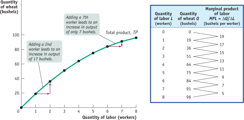
Figure 54.1: The Production Function and the Total Product Curve for George and Martha’s FarmThe table shows the production function, the relationship between the quantity of the variable input (labor, measured in number of workers) and the quantity of output (wheat, measured in bushels) for a given quantity of the fixed input. It also shows the marginal product of labor on George and Martha’s farm. The total product curve shows the production function graphically. It slopes upward because more wheat is produced as more workers are employed. It also becomes flatter because the marginal product of labor declines as more and more workers are employed.

The marginal product of an input is the additional quantity of output produced by using one more unit of that input.

547

Although the total product curve in Figure 54.1 slopes upward along its entire length, the slope isn’t constant: as you move up the curve to the right, it flattens out. To understand this changing slope, look at the third column of the table in Figure 54.1, which shows the change in the quantity of output generated by adding one more worker. That is, it shows the marginal product of labor, or MPL: the additional quantity of output from using one more unit of labor (one more worker).

AP® Exam Tip

Whatever units you choose to use in marginal analysis, always be careful that you use the same units throughout the problem.

In this example, we have data at intervals of 1 worker—that is, we have information on the quantity of output when there are 3 workers, 4 workers, and so on. Sometimes data aren’t available in increments of 1 unit—for example, you might have information on the quantity of output only when there are 40 workers and when there are 50 workers. In this case, you can use the following equation to calculate the marginal product of labor:

Recall that △, the Greek uppercase delta, represents the change in a variable. Now we can explain the significance of the slope of the total product curve: it is equal to the marginal product of labor. The slope of a line is equal to “rise” over “run.” This implies that the slope of the total product curve is the change in the quantity of output (the “rise”) divided by the change in the quantity of labor (the “run”). And, as we can see from Equation 54-1, this is simply the marginal product of labor. So in Figure 54.1, the fact that the marginal product of the first worker is 19 also means that the slope of the total product curve in going from 0 to 1 worker is 19. Similarly, the slope of the total product curve in going from 1 to 2 workers is the same as the marginal product of the second worker, 17, and so on.

Was Malthus Right?

In 1798, Thomas Malthus, an English pastor, introduced the principle of diminishing returns to an input. Malthus’s writings were influential in his own time and continue to provoke heated argument to this day.

Malthus argued that as a country’s population grew but its land area remained fixed, it would become increasingly difficult to grow enough food. Though more intensive cultivation of the land could increase yields, as the marginal product of labor declined, each successive farmer would add less to the total than the last.

From this argument, Malthus drew a powerful conclusion—that misery was the normal condition of humankind. In a country with a small population and abundant land (a description of the United States at the time), he argued, families would be large and the population would grow rapidly. Ultimately, the pressure of population on the land would reduce the condition of most people to a level at which starvation and disease held the population in check. (Arguments like this led the historian Thomas Carlyle to dub economics the “dismal science.”)

Happily, over the long term, Malthus’s predictions have turned out to be wrong. World population has increased from about 1 billion when Malthus wrote to more than 7.2 billion in 2014, but in most of the world people eat better now than ever before. So was Malthus completely wrong? And do his incorrect predictions refute the idea of diminishing returns? No, on both counts.

First, the Malthusian story is a pretty accurate description of 57 of the last 59 centuries: peasants in eighteenth-century France probably did not live much better than Egyptian peasants in the age of the pyramids. Yet diminishing returns does not mean that using more labor to grow food on a given amount of land will lead to a decline in the marginal product of labor—if there is also a radical improvement in farming technology. Fortunately, since the eighteenth century, technological progress has been so rapid that it has alleviated much of the limits imposed by diminishing returns. Diminishing returns implies that the marginal product declines when all other things—including technology—remain the same. So the happy fact that Malthus’s predictions were wrong does not invalidate the concept of diminishing returns.

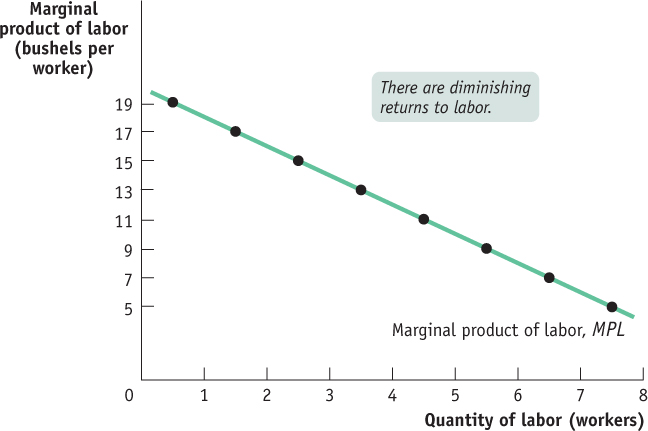
In this example, the marginal product of labor steadily declines as more workers are hired—that is, each successive worker adds less to output than the previous worker. So as employment increases, the total product curve gets flatter.

Figure 54.2 shows how the marginal product of labor depends on the number of workers employed on the farm. The marginal product of labor, MPL, is measured on the vertical axis in units of physical output—bushels of wheat—produced per additional worker, and the number of workers employed is measured on the horizontal axis. You can see from the table in Figure 54.1 that if 5 workers are employed instead of 4, output rises from 64 to 75 bushels; in this case the marginal product of labor is 11 bushels—the same number found in Figure 54.2. To indicate that 11 bushels is the marginal product when employment rises from 4 to 5, we place the point corresponding to that information halfway between 4 and 5 workers.

There are diminishing returns to an input when an increase in the quantity of that input, holding the levels of all other inputs fixed, leads to a decline in the marginal product of that input.

548

In this example the marginal product of labor falls as the number of workers increases. That is, there are diminishing returns to labor on George and Martha’s farm. In general, there are diminishing returns to an input when an increase in the quantity of that input, holding the quantity of all other inputs fixed, reduces that input’s marginal product. Due to diminishing returns to labor, the MPL curve is negatively sloped.

To grasp why diminishing returns can occur, think about what happens as George and Martha add more and more workers without increasing the number of acres. As the number of workers increases, the land is farmed more intensively and the number of bushels increases. But each additional worker is working with a smaller share of the 10 acres—the fixed input—than the previous worker. As a result, the additional worker cannot produce as much output as the previous worker. So it’s not surprising that the marginal product of the additional worker falls.

The next module explains that opportunities for specialization among workers can allow the marginal product of labor to increase for the first few workers, but eventually diminishing returns set in as the result of redundancy and congestion. The crucial point to emphasize about diminishing returns is that, like many propositions in economics, it is an “other things equal” proposition: each successive unit of an input will raise production by less than the last if the quantity of all other inputs is held fixed.

Figure 54.2: The Marginal Product of Labor Curve for George and Martha’s FarmThe marginal product of labor curve plots each worker’s marginal product, the increase in the quantity of output generated by each additional worker. The change in the quantity of output is measured on the vertical axis and the number of workers employed on the horizontal axis. The first worker employed generates an increase in output of 19 bushels, the second worker generates an increase of 17 bushels, and so on. The curve slopes downward due to diminishing returns to labor.

With diminishing returns to labor, as more and more workers are added to a fixed amount of land, each worker adds less to total output than the previous worker.

Photodisc

549

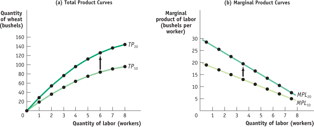
What would happen if the levels of other inputs were allowed to change? You can see the answer illustrated in Figure 54.3. Panel (a) shows two total product curves, TP₁₀ and TP₂₀. TP₁₀ is the farm’s total product curve when its total area is 10 acres (the same curve as in Figure 54.1). TP₂₀ is the total product curve when the farm’s area has increased to 20 acres. Except when 0 workers are employed, TP₂₀ lies everywhere above TP₁₀ because with more acres available, any given number of workers produces more output. Panel (b) shows the corresponding marginal product of labor curves. MPL₁₀ is the marginal product of labor curve given 10 acres to cultivate (the same curve as in Figure 54.2), and MPL₂₀ is the marginal product of labor curve given 20 acres. Both curves slope downward because, in each case, the amount of land is fixed, albeit at different levels. But MPL₂₀ lies everywhere above MPL₁₀, reflecting the fact that the marginal product of the same worker is higher when he or she has more of the fixed input to work with.

AP® Exam Tip

The MPL typically falls as more workers are hired because increases in production are limited by a fixed amount of capital that must be shared among the growing number of workers. Also, it may be necessary to hire less qualified workers.

Figure 54.3 demonstrates a general result: the position of the total product curve depends on the quantities of other inputs. If you change the quantities of the other inputs, both the total product curve and the marginal product curve of the remaining input will shift. The importance of the “other things equal” assumption in discussing diminishing returns is illustrated in the FYI.

Figure 54.3: Total Product, Marginal Product, and the Fixed InputThis figure shows how the quantity of output—illustrated by the total product curve—and marginal product depend on the level of the fixed input. Panel (a) shows two total product curves for George and Martha’s farm, TP₁₀ when their farm is 10 acres and TP₂₀ when it is 20 acres. With more land, each worker can produce more wheat. So an increase in the fixed input shifts the total product curve up from TP₁₀ to TP₂₀. This also implies that the marginal product of each worker is higher when the farm is 20 acres than when it is 10 acres. As a result, an increase in acreage also shifts the marginal product of labor curve up from MPL₁₀ to MPL₂₀. Panel (b) shows the marginal product of labor curves. Note that both marginal product of labor curves still slope downward due to diminishing returns to labor.