From the Production Function to Cost Curves
Now that we have learned about the firm’s production function, we can use that knowledge to develop its cost curves. To see how a firm’s production function is related to its cost curves, let’s turn once again to George and Martha’s farm. Once George and Martha know their production function, they know the relationship between inputs of labor and land and output of wheat. But if they want to maximize their profits, they need to translate this knowledge into information about the relationship between the quantity of output and cost. Let’s see how they can do this.
AP® Exam Tip
Understanding cost curves is crucial to understanding the market structure models in the coming sections. Create note cards with definitions and formulas from this module to aid you in your studies.
A fixed cost is a cost that does not depend on the quantity of output produced. It is the cost of the fixed input.
To translate information about a firm’s production function into information about its cost, we need to know how much the firm must pay for its inputs. We will assume that George and Martha face either an explicit or an implicit cost of $400 for the use of the land. As we learned previously, it is irrelevant whether George and Martha must rent the land for $400 from someone else or whether they own the land themselves and forgo earning $400 from renting it to someone else. Either way, they pay an opportunity cost of $400 by using the land to grow wheat. Moreover, since the land is a fixed input for which George and Martha pay $400 whether they grow one bushel of wheat or one hundred, its cost is a fixed cost, denoted by FC—a cost that does not depend on the quantity of output produced. In business, a fixed cost is often referred to as an “overhead cost.”
A variable cost is a cost that depends on the quantity of output produced. It is the cost of the variable input.
The total cost of producing a given quantity of output is the sum of the fixed cost and the variable cost of producing that quantity of output.
We also assume that George and Martha must pay each worker $200. Using their production function, George and Martha know that the number of workers they must hire depends on the amount of wheat they intend to produce. So the cost of labor, which is equal to the number of workers multiplied by $200, is a variable cost, denoted by VC—a cost that depends on the quantity of output produced. Adding the fixed cost and the variable cost of a given quantity of output gives the total cost, or TC, of that quantity of output. We can express the relationship among fixed cost, variable cost, and total cost as an equation:
(55-
or
TC = FC + VC
The table in Figure 55.1 shows how total cost is calculated for George and Martha’s farm. The second column shows the number of workers employed, L. The third column shows the corresponding level of output, Q, taken from the table in Figure 54.1. The fourth column shows the variable cost, VC, equal to the number of workers multiplied by $200. The fifth column shows the fixed cost, FC, which is $400 regardless of the quantity of wheat produced. The sixth column shows the total cost of output, TC, which is the variable cost plus the fixed cost.
| Figure 55.1 | The Total Cost Curve for George and Martha’s Farm |
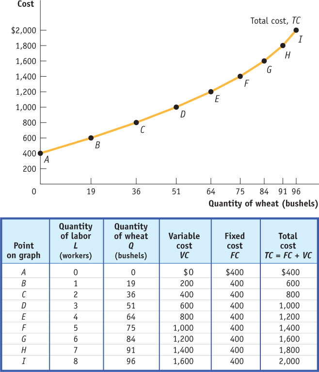
The total cost curve shows how total cost depends on the quantity of output.
The first column labels each row of the table with a letter, from A to I. These labels will be helpful in understanding our next step: drawing the total cost curve, a curve that shows how total cost depends on the quantity of output.
George and Martha’s total cost curve is shown in the diagram in Figure 55.1, where the horizontal axis measures the quantity of output in bushels of wheat and the vertical axis measures total cost in dollars. Each point on the curve corresponds to one row of the table in Figure 55.1. For example, point A shows the situation when 0 workers are employed: output is 0, and total cost is equal to fixed cost, $400. Similarly, point B shows the situation when 1 worker is employed: output is 19 bushels, and total cost is $600, equal to the sum of $400 in fixed cost and $200 in variable cost.
Like the total product curve, the total cost curve slopes upward: due to the increasing variable cost, the more output produced, the higher the farm’s total cost. But unlike the total product curve, which gets flatter as employment rises, the total cost curve gets steeper. That is, the slope of the total cost curve is greater as the amount of output produced increases. As we will soon see, the steepening of the total cost curve is also due to diminishing returns to the variable input. Before we can see why, we must first look at the relationships among several useful measures of cost.