Tackle the Test: Free-Response Questions
Question
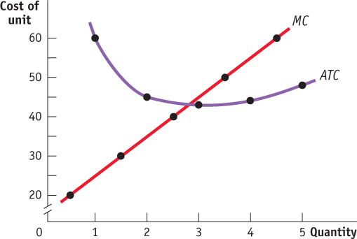
Use the information in the table below to answer the following questions.
Quantity Variable cost Total cost 0 $0 $40 1 20 60 2 50 90 3 90 130 4 140 180 5 200 240 What is the firm’s level of fixed cost? Explain how you know.
Draw one correctly labeled graph showing the firm’s marginal and average total cost curves.
Rubric for FRQ 1 (6 points)
1 point: FC = $40
1 point: We can identify the fixed cost as $40 because when the firm is not producing, it still incurs a cost of $40. This could only be the result of a fixed cost because variable cost is zero when output is zero.
1 point: Graph with correct labels (“Cost of unit” on vertical axis; “Quantity” on horizontal axis)
1 point Upward-
sloping MC curve plotted according to data, labeled “MC” 1 point: U-
shaped ATC curve plotted according to the provided data, labeled “ATC” 1 point: MC curve crossing at minimum of ATC curve (Note: We have simplified this graph by drawing smooth lines between discrete points. If we had drawn the MC curve as a step function instead, the MC curve would have crossed the ATC curve exactly at its minimum point.)
Question
Draw a correctly labeled graph showing a firm with a realistic “swoosh-
shaped” MC curve and ATC, AVC, and AFC curves with their usual shapes. (6 points) Rubric for FRQ 2 (6 points)
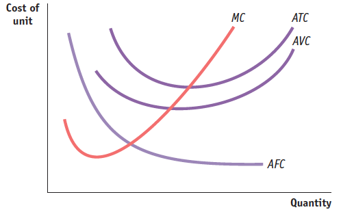
1 point: Graph labeled “Cost of unit” or “Dollars per unit” on the vertical axis and “Quantity” or “Q” on the horizontal axis
1 point: Swoosh-shaped MC curve labeled “MC”
1 point: U-shaped ATC curve labeled “ATC”
1 point: U-shaped AVC curve that is below the ATC curve and is labeled “AVC”
1 point: Downward-sloping AFC curve that is below the ATC curve and is labeled “AFC”
1 point: The MC curve intersects the minimum points of the ATC curve and the AVC curve.