Check Your Understanding

1. Question

   Which of the following events will induce firms to enter an industry? Which will induce firms to exit? When will entry or exit cease? Explain your answers.

   1. A technological advance lowers the fixed cost of production of every firm in the industry.

      When fixed costs fall, ATC decreases and each firm’s profit at the current output level increases. In the long run, new firms will enter the industry. This increase in supply drives down price and profits. Once profits are driven back to zero, entry will cease.

   2. The wages paid to workers in the industry go up for an extended period of time.

      An increase in wages means that AVC and ATC increase. In the short run, some firms incur losses. As a result, in the long run, some firms will exit the industry. As firms exit, supply decreases, price rises, and losses are reduced. Exit will cease once losses return to zero.

   3. A permanent change in consumer tastes increases demand for the good.

      Price increases as demand increases, leading to short-run profits. In the long run, firms will enter the industry, generating an increase in supply, a fall in price, and a fall in profits. Once profits are driven back to zero, entry will cease.

   4. The price of a key input rises due to a long-term shortage of that input.

      The shortage of inputs causes resource price to increase, increasing AVC and ATC. Firms incur losses in the short run, and some firms will exit the industry in the long run. The fall in supply means an increase in price and a reduction in losses. Exit will cease once losses return to zero.

2. Question

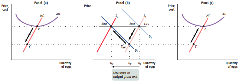
   Assume that the egg industry is perfectly competitive and is in long-run equilibrium with a perfectly elastic long-run industry supply curve. Health concerns about cholesterol then lead to a decrease in demand. Construct a figure similar to Figure 60.3, showing the short-run behavior of the industry and how long-run equilibrium is reestablished.

   In the accompanying diagram, point X_MKT in panel (b), the intersection of S₁ and D₁ , represents the long-run industry equilibrium before the change in consumer tastes. When tastes change, demand falls and the industry moves in the short run to point Y_MKT in panel (b), at the intersection of the new demand curve D₂ and S₁ , the short-run supply curve representing the same number of egg producers as in the original equilibrium at point X_MKT . As the market price falls, each individual firm reacts by producing less–shown in panel (a) as the movement from point X to point Y–so long as the market price remains above the minimum average variable cost. If market price falls below minimum average variable cost, the firm would shut down immediately. At point Y_MKT , the price of eggs is below minimum average total cost, creating losses for producers. This leads some firms to exit, which shifts the short-run industry supply curve leftward to S₂ . A new long-run equilibrium is established at point Z_MKT . As this occurs, the market price rises again, and as shown in panel (c), each remaining producer reacts by increasing output (here, from point Y to point Z ). All remaining producers again make zero profit. The decrease in the quantity of eggs supplied in the industry comes entirely from the exit of some producers from the industry. The long-run industry supply curve is the curve labeled LRS in panel (b).