In the previous module we used a labor market example to explain why a firm’s individual demand curve for a factor is its marginal revenue product curve. Now we look at the distinguishing characteristics of demand and supply in land and capital markets, and how the equilibrium price and quantity of these factors are determined.

The result that we derived for demand in the labor market also applies to other factors of production. For example, suppose that a farmer is considering whether to rent an additional acre of land for the next year. He or she will compare the cost of renting that acre with the additional revenue generated by employing an additional acre—the marginal revenue product of an acre of land. To maximize profit, the farmer will rent more land up until the marginal revenue product of an acre of land is equal to the rental cost per acre. The same is true for capital: the decision of whether to rent an additional piece of equipment comes down to a comparison of the additional cost of the equipment with the additional revenue it generates.

What if the farmer already owns the land or the firm already owns the equipment? As discussed in Module 52 in the context of Babette’s Cajun Café, even if you own land or capital, there is an implicit cost—the opportunity cost—of using it for a given activity because it could be used for something else, such as renting it out to other firms at the market rental rate. So a profit-maximizing firm employs additional units of land and capital until the cost of the last unit employed, explicit or implicit, is equal to the marginal revenue product of that unit. We call the explicit or implicit cost of using a unit of land or capital for a set period of time its rental rate.

As with labor, due to diminishing returns, the marginal revenue product curve and therefore the individual firm’s demand curves for land and capital slope downward.

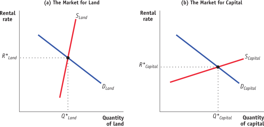
Figure 70.1 illustrates the markets for land and capital. The red curve in panel (a) is the supply curve for land. As we have drawn it, the supply curve for land is relatively steep and therefore relatively inelastic. This reflects the fact that finding new supplies of land for production is typically difficult and expensive—for example, creating new farmland through expensive irrigation.

The red curve in panel (b) is the supply curve for capital. In contrast to the supply curve for land, the supply curve for capital is relatively flat and therefore relatively elastic. That’s because the supply of capital is relatively responsive to price: capital is typically paid for with the savings of investors, and the amount of savings that investors make available is relatively responsive to the rental rate for capital.

As in the case of supply curves for goods and services, the supply curve for a factor of production will shift as the factor becomes more or less available. For example, the supply of farmland could decrease as a result of a drought or the supply of capital could increase as a result of a government policy to promote investment. Because of diminishing returns, when the supply of land or capital changes, its marginal product will change. When the supply of land or capital decreases, the marginal product and rental rate increase. For example, if the number of available delivery trucks decreased, the additional benefit from the last truck used would be higher than before—it would serve more critical delivery needs—and firms would pay more for it. Likewise, when the supply of land or capital increases, the marginal product and rental rate decrease.

The equilibrium rental rate and quantity in the land and capital markets are found at the intersection of the supply and demand curves in Figure 70.1. Panel (a) shows the equilibrium in the market for land. Summing all of the firm demand curves for land gives us the market demand curve for land. The equilibrium rental rate for land is R*_Land, and the equilibrium quantity of land employed in production is Q*_Land. In a competitive land market, each unit of land will be paid the equilibrium marginal revenue product of land. The equilibrium marginal revenue product of a factor is the additional revenue generated by the last unit of that factor employed in the entire market for that factor.

Panel (b) shows the equilibrium in the market for capital. The equilibrium rental rate for capital is R*_Capital, and the equilibrium quantity of capital employed in production is Q*_Capital. In a competitive capital market, each unit of capital will be paid the equilibrium marginal revenue product of capital.

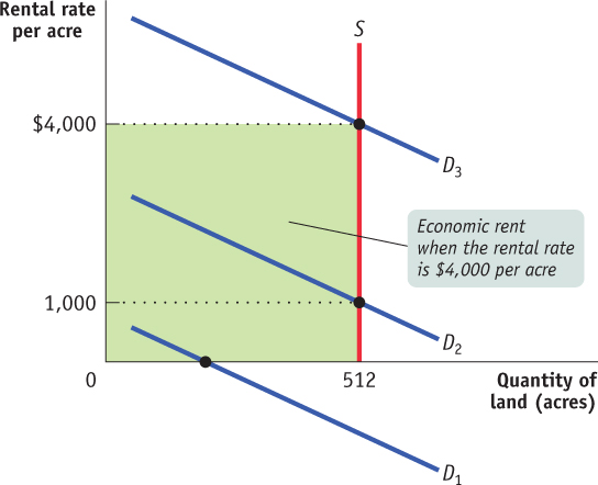
When the payment for a factor of production is higher than it would need to be to employ that factor, the factor is earning economic rent. Consider the 512 acres of flat land in Ouray, Colorado, which is ringed by mountains too steep to build or farm on. Because the land is in fixed supply, the supply curve is vertical as shown in Figure 70.2, and the monthly rental rate is determined by the level of demand. The land would be there even if the rental rate were zero, as it would be if the demand curve were D₁. Since no payment is needed to make the land available, the entire payment for the land is economic rent. If the demand curve were D₂, the rental rate would be $1,000 an acre, and the economic rent would be $1,000 × 512 = $512,000. If the demand curve were D₃, the rental rate would be $4,000 per acre, and the economic rent would be $4,000 × 512 = $2,480,000.

The appropriate distribution of the economic rent from land is a source of debate. Socialists argue that land should be publicly owned so that its benefits can be shared broadly. Critics argue that markets provide incentives for resources to be allocated to their most productive uses, whereas publicly owned land might not be allocated with the same attention to opportunity costs.

With private land ownership, portions of the economic rent can be redistributed using a land tax, which creates no deadweight loss when land is in fixed supply. Recall that many types of taxes cause deadweight loss by reducing the equilibrium quantity and eliminating some mutually beneficial exchanges. When the quantity of land is fixed, a tax on land does not decrease the quantity of land that is bought and sold, so there is no deadweight loss. The entire burden of the tax is placed on landowners in the form of a loss of economic rent. Although a land tax is appealing from an efficiency standpoint, there is no consensus on the level of taxation that is fair to landowners.

Workers receive economic rent as well. If you earn $12 per hour, but you would be willing to work for as little as $8 per hour—perhaps because that’s the most you could earn elsewhere—you receive $4 of economic rent per hour. If you don’t have any alternatives and you love your job so much that you would work for free, your income is pure economic rent.

Now that we know how equilibrium rental rates and quantities are determined in factor markets, we can learn how these markets influence the factor distribution of income. To do this, we look more closely at marginal productivity in factor markets.