MODULE 71: The Market for Labor

Equilibrium in the Labor Market

Now that we have discussed the labor supply curve, we can use the supply and demand curves for labor to determine the equilibrium wage and level of employment in the labor market.

709

The Decline of the Summer Job

Come summertime, resort towns along the New Jersey shore find themselves facing a recurring annual problem: a serious shortage of lifeguards. Traditionally, lifeguard positions, together with many other seasonal jobs, have been filled mainly by high school and college students. But in recent years a growing number of young Americans have chosen not to take summer jobs. In 1979, 71% of Americans between the ages of 16 and 19 were in the summer workforce. Twenty years later that number had fallen to 63%; and by 2013, it was 34.5%. Data show that young men in particular have become much less willing to take summer jobs.

One explanation for the decline in the summer labor supply is that more students feel they should devote their summers to additional study. But an important factor in the decline is increasing household affluence. As a result, many teenagers no longer feel pressured to contribute to household finances by taking a summer job; that is, the income effect leads to a reduced labor supply. Another factor points to the substitution effect: increased competition from immigrants, who are now doing the jobs typically done by teenagers (mowing lawns, delivering pizzas), has led to a decline in wages. So many teenagers forgo summer work and consume leisure instead.

Source: Bureau of Labor Statistics.

Figure 71.2 illustrates the labor market as a whole. The market labor demand curve, like the market demand curve for a good, is the horizontal sum of all the individual labor demand curves of all the firms that hire labor. And recall that a firm’s labor demand curve is the same as its marginal revenue product of labor curve. As discussed above, the labor supply curve is upward-sloping.

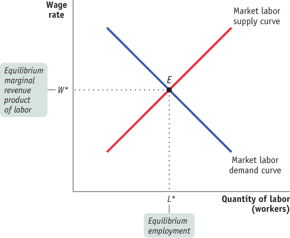
Figure 71.2: Equilibrium in the Labor MarketThe market labor demand curve is the horizontal sum of the individual labor demand curves of all producers. Here the equilibrium wage rate is W*, the equilibrium employment level is L*, and every producer hires labor up to the point at which MRPL = W*. So labor is paid its equilibrium marginal revenue product, that is, the marginal revenue product of the last worker hired in the labor market as a whole.

The equilibrium wage rate is the wage rate at which the quantity of labor supplied is equal to the quantity of labor demanded. In Figure 71.2, this leads to an equilibrium wage rate of W* and the corresponding equilibrium employment level of L*. The equilibrium wage rate is also known as the market wage rate.

So far we have assumed that the labor market is perfectly competitive, but that isn’t always the case. Next we’ll examine the workings of an imperfectly competitive labor market.

When the Labor Market Is Not Perfectly Competitive

710

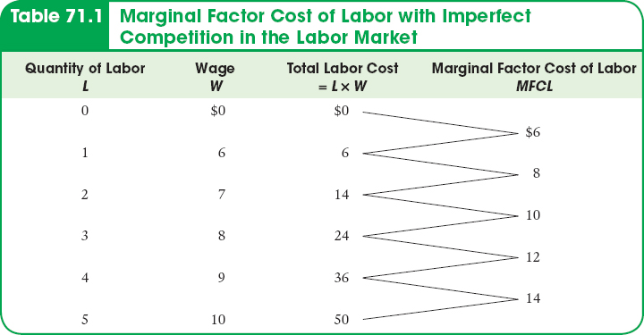
The marginal factor cost is the additional cost of employing an additional unit of a factor of production.

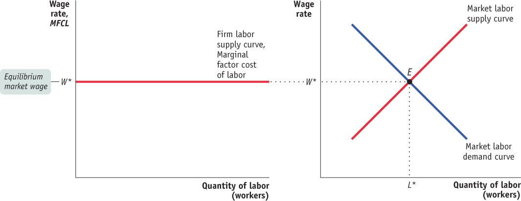
There are important differences when considering an imperfectly competitive factor market rather than a perfectly competitive market. One major difference is the marginal factor cost. The marginal factor cost is the additional cost of employing one more unit of a factor of production. For example, the marginal factor cost of labor (MFCL) is the additional cost of hiring one more unit of labor. With perfect competition in the labor market, each firm is so small that it can hire as much labor as it wants at the market wage. The firm’s hiring decision does not affect the market. This means that with perfect competition in the labor market, the additional cost of hiring another worker (the MFCL) is always equal to the market wage, and each firm faces a horizontal labor supply curve, as shown in Figure 71.3.

Figure 71.3: Firm Labor Supply in a Perfectly Competitive Labor MarketIn a perfectly competitive labor market, an individual firm faces a labor supply curve that is horizontal at the market equilibrium wage because the firm is so small relative to the market that it can hire all the labor that it wants at the market wage. For this reason, the labor supply curve for a firm in a perfectly competitive labor market is equivalent to the marginal factor cost of labor curve.

A monopsonist is a single buyer in a factor market. A market in which there is a monopsonist is a monopsony.

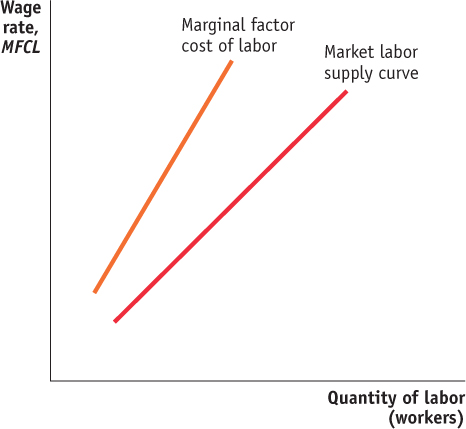
A firm faces a very different labor supply curve in a labor market characterized by imperfect competition: it is upward-sloping and the marginal factor cost is above the market wage. Unlike a perfect competitor that is small and cannot affect the market, a firm in an imperfectly competitive labor market is large enough to affect the market wage. For example, a labor market in which there is only one firm hiring labor is called a monopsony. A monopsonist is the single buyer of a factor. Perhaps you’ve seen a small town where one firm, such as a meatpacking company or a lumber mill, hires most of the labor—that’s an example of a monopsony. Since the firm already hires most of the available labor in the town, if it wants to hire more workers it has to offer higher wages to attract them. The higher wages go to all workers, not just the workers hired last. Therefore, the additional cost of hiring an additional worker (MFCL) is higher than the wage: it is the wage plus the raises paid to all workers. The calculation of MFCL is shown in Table 71.1.

The fact that a firm in an imperfectly competitive labor market must raise the wage to hire more workers means that the MFCL curve is above the labor supply curve, as shown in Figure 71.4. The explanation for this is similar to the explanation for why the monopolist’s marginal revenue curve is below the demand curve. To sell one more, the monopolist has to lower the price, so the additional revenue is the price minus the losses on the units that would otherwise sell at the higher price. Here, to hire an additional worker, the monopolist has to raise the wage, so the marginal factor cost is the wage plus the wage increase for those workers who could otherwise be hired at the lower wage.

Figure 71.4: Supply of Labor and Marginal Factor Cost in an Imperfectly Competitive MarketThe marginal factor cost of labor curve is above the market labor supply curve because, to hire more workers in an imperfectly competitive labor market (such as a monopsony), the firm must raise the wage and pay everyone more. This makes the additional cost of hiring another worker higher than the wage rate.

711

Equilibrium in the Imperfectly Competitive Labor Market

In a perfectly competitive labor market, firms hire labor until the marginal revenue product of labor equals the market wage. With imperfect competition in a factor market, a firm will hire additional workers until the marginal revenue product of labor equals the marginal factor cost of labor. Note that the marginal factor cost of labor in a perfectly competitive labor market is the market wage, so the term marginal factor cost is generally applicable to the analysis of hiring decisions in both perfectly competitive and imperfectly competitive labor markets. The term we used previously, wage, only applies in the specific case of perfect competition in the labor market. Thus, we can generalize and say that every firm hires workers up to the point at which the marginal revenue product of labor equals the marginal factor cost of labor:

712

(71-1) Hire workers until MRPL = MFCL

Equilibrium in the labor market with imperfect competition is shown in Figure 71.5. Once an imperfectly competitive firm has determined the optimal number of workers to hire, L*, it finds the wage necessary to hire that number of workers by starting at the point on the labor supply curve above the optimal number of workers, and looking straight to the left to see the wage level at that point, W*.

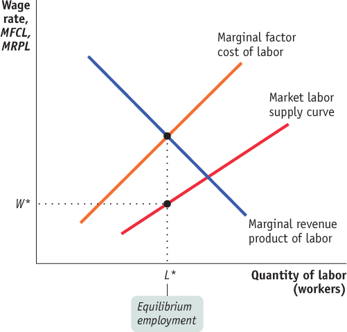
Figure 71.5: Equilibrium in the Labor Market with Imperfect CompetitionThe equilibrium quantity of labor is found where the marginal revenue product of labor equals the marginal factor cost, at L*. The equilibrium wage, W*, is found on the vertical axis at the height of the market supply curve directly above L*.

Let’s put the information we just learned together, again referring to Figure 71.5: In an imperfectly competitive labor market, the firm must offer a higher wage to hire more workers, so the marginal factor cost curve is above the labor supply curve. The equilibrium quantity of labor is found where the marginal revenue product equals the marginal factor cost, as represented by L* on the graph. The firm will pay the wage required to hire L* workers, which is found on the supply curve above L*. The labor supply curve shows that the quantity of labor supplied is equal to L* at a wage of W*. The equilibrium wage in the market is thus W*. Note that, unlike the wage in a perfectly competitive labor market, the wage in the imperfectly competitive labor market is less than the marginal factor cost of labor.

In Modules 69–71 we have learned how firms determine the optimal amount of land, labor, or capital to hire in factor markets. But often there are different combinations of factors that a firm can use to produce the same level of output. In the next module, we look at how a firm chooses between alternative input combinations for producing a given level of output.