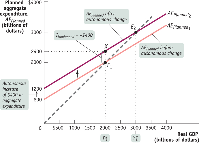
Figure11-10The Multiplier This figure illustrates the change in Y* caused by an autonomous increase in planned aggregate expenditure. The economy is initially at equilibrium point E1 with an income– expenditure equilibrium GDP,  , equal to 2000. An auto
n- omous increase in AEPlanned of 400 shifts the planned aggregate expenditure line upward by 400. The economy is no longer in income– expenditure equilibrium: real GDP is equal to 2000 but AEPlanned is now 2400, represented by point X. The vertical distance between the two planned aggregate expenditure lines, equal to 400, represents IUnplanned = −400—the negative inventory investment that the economy now experiences. respond by increasing production, and the economy eventually reaches a new income– expenditure equilibrium at E2 with a higher level of income– expenditure equilibrium GDP,  , equal to 3000.
, equal to 2000. An auto, equal to 3000.[Leave] [Close]