The Demand Curve
The law of demand says that, other things equal, a higher price for a good or service leads people to demand a smaller quantity of that good or service. On a graph, this means the demand curve is a downward sloping function of the price of the good or service being studied. For each quantity, the demand curve reveals the maximum price consumers are willing (and able) to pay. Similarly, at each level of the price, the demand curve reveals the maximum quantity that consumers are willing (and able) to purchase. In the case of a linear expression, a demand curve in its simplest form would be:
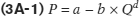
where P is the price, Qd is the quantity, and a and b are positive constants.1 That b × Qd is subtracted from a constant tells us the law of demand holds here—
Although Equation 3A-

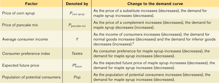
with a expanded to include several factors multiplied by constants that are summarized in Table 3A-1. These factors are all multiplied by positive constants that, like b, describe how sensitive the demand curve is to changes in those factors. The constant a0 picks up the impact of all other determinants of the demand for maple syrup that have been left out of the equation of the demand curve.
Note that the “other things equal” assumption means that everything in the demand curve equation, except P and Qd, are being held constant. So, other things equal, when we move along the demand curve as P and Qd change—
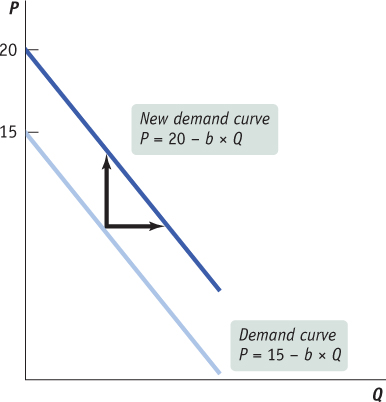
Note that if demand decreases (i.e., a decreases), the demand curve shifts down (or to the left).
Let us simplify the expanded equation. Suppose the following values apply for factors that affect the demand curve for maple syrup: Pcorn syrup = $10, Ppancake mix = $5, Y = $40, which represents the average income of a Canadian (in thousands of dollars), Tastes = 9,  = $20 (per litre), and Pop = 34, which is the population of Canada (in millions of people). Suppose also the values for the constants are a0 = $5, a1 = 0.25, a2 = 2, a3 = 0.5, a4 = $0.45, a5 = 1.5, a6 = $0.05, and b = 1.25.
Given these assumed values, the demand curve for maple syrup becomes:
