13.2 Fiscal Policy and the Multiplier
An expansionary fiscal policy, like the 2009 Economic Action Plan, pushes the aggregate demand curve to the right. A contractionary fiscal policy, like Minister of Finance Paul Martin’s 1995 federal spending cuts under Prime Minister Jean Chrétien, pushes the aggregate demand curve to the left. For policy-
Multiplier Effects of an Increase in Government Purchases of Goods and Services
Suppose that a government decides to spend $50 billion building bridges and roads. The government’s purchases of goods and services will directly increase total spending on final goods and services by $50 billion. But as we learned in Chapter 11, there will also be an indirect effect: the government’s purchases will start a chain reaction throughout the economy. The firms that produce the goods and services purchased by the government earn revenues that flow to households in the form of wages, profits, interest, and rent. This increase in disposable income leads to a rise in consumer spending. The rise in consumer spending, in turn, induces firms to increase output, leading to a further rise in disposable income, which leads to another round of consumer spending increases, and so on.
As we know, the multiplier is the ratio of the change in real GDP caused by an autonomous change in aggregate expenditure to the size of that autonomous change. An increase in government purchases of goods and services is a prime example of such an autonomous increase in aggregate expenditure.
In Chapter 11 we considered a simple case in which there are no taxes or international trade, so that any change in GDP accrues entirely to households. We also assumed that the aggregate price level is fixed, so that any increase in nominal GDP is also a rise in real GDP, and that the interest rate is fixed. In that case the multiplier is 1/(1 − MPC). Recall that MPC is the marginal propensity to consume, the fraction of an additional dollar in disposable income that is spent. For example, if the marginal propensity to consume is 0.5, the multiplier is 1/(1−0.5) = 1/0.5 = 2. Given a multiplier of 2, a $50 billion increase in government purchases of goods and services would increase real GDP by $100 billion. Of that $100 billion, $50 billion is the initial effect from the increase in G, and the remaining $50 billion is the subsequent effect arising from the increase in consumer spending.3
What happens if government purchases of goods and services are instead reduced? The math is exactly the same, except that there’s a minus sign in front: if government purchases of goods and services fall by $50 billion and the marginal propensity to consume is 0.5, real GDP falls by $100 billion.
Multiplier Effects of Changes in Government Transfers and Taxes
Expansionary or contractionary fiscal policy need not take the form of changes in government purchases of goods and services. Governments can also change transfer payments or taxes. In general, however, a change in government transfers or taxes shifts the aggregate demand curve by less than an equal-
To see why, imagine that instead of spending $50 billion on building bridges, the government simply hands out $50 billion in the form of government transfers. In this case, there is no direct effect on aggregate demand, as there was with government purchases of goods and services. Real GDP goes up only because households spend some of that $50 billion—
Table 13-1 shows a hypothetical comparison of two expansionary fiscal policies assuming an MPC equal to 0.5 and a multiplier equal to 2: one in which the government directly purchases $50 billion in goods and services and one in which the government makes transfer payments instead, sending out $50 billion in cheques to consumers. In each case there is a first-
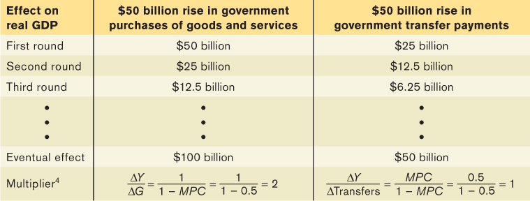
However, the first-
Overall, when expansionary fiscal policy takes the form of a rise in transfer payments, real GDP may rise by either more or less than the initial government outlay—
A tax cut has an effect similar to the effect of a transfer. It increases disposable income, leading to a series of increases in consumer spending. But the overall effect is smaller than that of an equal-
Lump-sum taxes are taxes that don’t depend on the taxpayer’s income.
We should also note that taxes introduce a further complication—
In practice, economists often argue that the size of the multiplier determines who among the population should get tax cuts or increases in government transfers. For example, compare the effects of an increase in employment insurance benefits with a cut in taxes on profits distributed to shareholders as dividends. Consumer surveys suggest that the average unemployed worker will spend a higher share of any increase in his or her disposable income than would the average recipient of dividend income. That is, people who are unemployed tend to have a higher MPC than people who own a lot of stocks because the latter tend to be wealthier and tend to save more of any increase in disposable income. If that’s true, a dollar spent on employment insurance benefits increases aggregate demand more than a dollar’s worth of dividend tax cuts.
How Taxes Affect the Multiplier
When we introduced the analysis of the multiplier in Chapter 11, we simplified matters by assuming that a $1 increase in real GDP raises disposable income by $1. In fact, however, government taxes capture some part of the increase in real GDP that occurs in each round of the multiplier process, since most government taxes depend positively on real GDP. As a result, disposable income increases by considerably less than $1 once we include non-
The increase in government tax revenue when real GDP rises isn’t the result of a deliberate decision or action by the government. It’s a consequence of the way the tax laws are written, which causes most sources of government revenue to increase automatically when real GDP goes up. For example, income tax receipts increase when real GDP rises because the amount each individual owes in taxes depends positively on his or her income, and households’ taxable income rises when real GDP rises. Sales tax receipts increase when real GDP rises because people with more income spend more on goods and services. And corporate profit tax receipts increase when real GDP rises because profits increase when the economy expands.
The effect of these automatic increases in tax revenue is to reduce the size of the multiplier. Remember, the multiplier is the result of a chain reaction in which higher real GDP leads to higher disposable income, which leads to higher consumer spending, which leads to further increases in real GDP. The fact that the government siphons off some of any increase in real GDP means that at each stage of this process, the increase in consumer spending is smaller than it would be if non-
Many macroeconomists believe it’s a good thing that in real life taxes reduce the multiplier. In Chapter 12 we argued that most, though not all, recessions are the result of negative demand shocks. The same mechanism that causes tax revenue to increase when the economy expands causes it to decrease when the economy contracts. Since tax receipts decrease when real GDP falls, the effects of these negative demand shocks are smaller than they would be if there were no taxes. The decrease in tax revenue reduces the adverse effect of the initial fall in aggregate demand—
Automatic stabilizers are government spending and taxation rules that cause fiscal policy to be automatically expansionary when the economy contracts and automatically contractionary when the economy expands.
The automatic decrease in government tax revenue generated by a fall in real GDP—
The rules that govern tax collection aren’t the only automatic stabilizers, although they are the most important ones. Some types of government transfers also play a stabilizing role. For example, more people receive employment insurance (EI) payments when the economy is depressed than when it is booming. The same is true of social assistance programs such as welfare, rent and daycare subsidies, and student assistance grants and loans. So transfer payments tend to rise when the economy is contracting and fall when the economy is expanding. Like changes in tax revenue, these automatic changes in transfers tend to reduce the size of the multiplier because the total change in disposable income that results from a given rise or fall in real GDP is smaller.
As in the case of government tax revenue, many macroeconomists believe that it’s a good thing that government transfers reduce the multiplier. Expansionary and contractionary fiscal policies that are the result of automatic stabilizers are widely considered helpful to macroeconomic stabilization because they blunt the extremes of the business cycle.
Discretionary fiscal policy is fiscal policy that is the result of deliberate actions by policy-
But what about fiscal policy that isn’t the result of automatic stabilizers? Discretionary fiscal policy is fiscal policy that is the direct result of deliberate actions by policy-

MULTIPLIERS AND THE 2009 ECONOMIC ACTION PLAN
Canada’s Economic Action Plan was the largest peacetime example of discretionary fiscal expansion in Canadian history. The total stimulus was about $62 billion, including all provincial and municipal contributions. But it wasn’t spent all at once: only about half, or roughly $29 billion, of the stimulus arrived in 2009, the year of peak impact. Still, even that was a lot—
The plan was released late in January 2009 and had three guiding principles. It was to be
timely, to help support the economy within the first 120 days when private demand was weakest;
targeted to Canadian businesses and families most in need so as to create the largest increase in Canadian jobs and output; and
temporary, so that the stimulus would be phased out by the time the economy recovered, thus avoiding long-
term deficits and/or overstimulating the economy.
Initial government estimates of the economic impact of the proposed plan were generated using the Department of Finance’s Canadian Economic and Fiscal Model (CEFM), a complex computer-
By May 2009, Parliamentary Budget Officer (PBO) Kevin Page had begun to question the government’s estimates as to the size and timing of the multipliers. He noted that in reality the multipliers varied, sometimes dramatically, across the various kinds of tax and spending options available. The PBO provided this table of estimated multipliers:
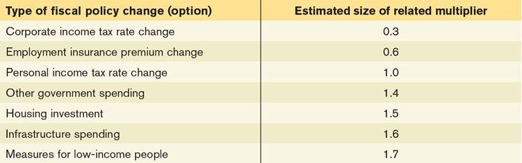
Notice that measures aimed at households and businesses generally have multiplier effects of 1.0 or less. This occurs since these measures are subject to a greater degree of “leakage.” That is, some of the change becomes a change in savings or in imports rather than a change in demand for domestically produced output. One notable exception is a measure aimed at low-

Other reservations were expressed, too. About three times more of the plan’s measures focused on areas with multipliers exceeding 1.0 than those with smaller multipliers. The fact that about one quarter of the stimulus spending was on measures with “small” multipliers led the PBO and others to question whether those most in need were truly being assisted. Critics, including the PBO, also questioned whether the plan could be “rolled out” on a timely basis. They noted that while housing investment and infrastructure projects do have high multiplier effects, these projects tend to start very slowly. Further, the government, hoping to have the plan rolled out within a two-
However, despite the reservations people had about the Plan, it seems to have succeeded. In February 2010, just over a year after the Plan was proposed, the Conference Board of Canada stated that these forecasts and their associated estimated impact on the economy were reasonable and conservative. That is, the assumed or estimated multiplier effects were not too aggressive and thus the estimated stimulus was not being overstated for the intended two-

Quick Review
The amount by which changes in government purchases raise real GDP is determined by the multiplier.
Changes in taxes and government transfers also move real GDP, but by less than equal-
sized changes in government purchases. Taxes reduce the size of the multiplier unless they are lump-sum taxes.
Taxes and some government transfers act as automatic stabilizers as tax revenue is positively correlated (that is, moves in the same direction) with changes in real GDP and some government transfers are negatively correlated with changes in real GDP. Many economists believe that it is a good thing that they reduce the size of the multiplier. In contrast, the use of discretionary fiscal policy is more controversial.
Check Your Understanding 13-2
CHECK YOUR UNDERSTANDING 13-2
Explain why a $500 million increase in government purchases of goods and services will generate a larger rise in real GDP than a $500 million increase in government transfers.
A $500 million increase in government purchases of goods and services directly increases aggregate expenditure by $500 million, which then starts the multiplier in motion. It will increase real GDP by $500 million × 1/(1 – MPC). A $500 million increase in government transfers increases aggregate expenditure only to the extent that it leads to an increase in consumer spending. Consumer spending rises by MPC × $1 for every $1 increase in disposable income, where MPC is less than 1. So a $500 million increase in government transfers will cause a rise in real GDP only MPC times as much as a $500 million increase in government purchases of goods and services. It will increase real GDP by $500 million × MPC/(1 – MPC).
Explain why a $500 million reduction in government purchases of goods and services will generate a larger fall in real GDP than a $500 million reduction in government transfers.
This is the same issue as in Problem 1, but in reverse. If government purchases of goods and services fall by $500 million, the initial fall in aggregate expenditure is $500 million. If there is a $500 million reduction in government transfers, the initial fall in aggregate expenditure is MPC × $500 million, which is less than $500 million.
The country of Boldovia has no employment insurance benefits and a tax system using only lump-
sum taxes. The neighbouring country of Moldovia has generous employment benefits and a tax system in which residents must pay a percentage of their income. Which country will experience greater variation in real GDP in response to demand shocks, positive and negative? Explain.
Boldovia will experience greater variation in its real GDP than Moldovia because Moldovia has automatic stabilizers while Boldovia does not. In Moldovia the effects of slumps will be lessened by unemployment insurance benefits that will support residents’ incomes, while the effects of booms will be diminished because tax revenues will go up. In contrast, incomes will not be supported in Boldovia during slumps because there is no unemployment insurance. In addition, because Boldovia has lump-