15.3 Monetary Policy and Aggregate Demand
In Chapter 13 we saw how fiscal policy can be used to stabilize the economy. Now we will see how monetary policy—
Expansionary and Contractionary Monetary Policy
In Chapter 12 we learned that monetary policy shifts the aggregate demand curve. We can now explain how that works: through the effect of monetary policy on the interest rate.
Expansionary monetary policy is monetary policy that increases aggregate demand.
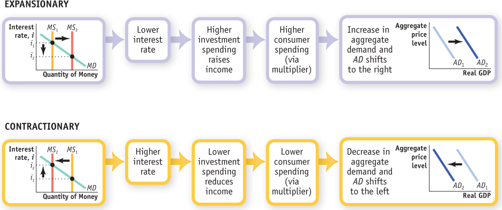
Figure 15-8 illustrates the process. Suppose, first, that the Bank of Canada wants to reduce interest rates, so it expands the money supply. As you can see in the top portion of the figure, a lower interest rate, will lead, other things equal, to more investment spending. This will in turn lead to higher consumer spending, through the multiplier process, and to an increase in aggregate output demanded. In the end, the total quantity of goods and services demanded at any given aggregate price level rises when the quantity of money increases, and the AD curve shifts to the right. Monetary policy that increases the demand for goods and services is known as expansionary monetary policy.
Suppose, alternatively, that the Bank of Canada wants to increase interest rates, so it contracts the money supply. You can see this process illustrated in the bottom portion of the diagram. Contraction of the money supply leads to a higher interest rate. The higher interest rate leads to lower investment spending, then to lower consumer spending, and then to a decrease in aggregate output demanded. So the total quantity of goods and services demanded falls when the money supply is reduced, and the AD curve shifts to the left. Monetary policy that decreases the demand for goods and services is called contractionary monetary policy.
Contractionary monetary policy is monetary policy that decreases aggregate demand.
Monetary Policy in Practice
How does the Bank of Canada decide whether to use expansionary or contractionary monetary policy? And how does it decide how much is enough? In Chapter 6 we learned that policy-
Typically, the Bank of Canada, like most central banks around the world, tends to engage in expansionary monetary policy when the economy is experiencing a recessionary gap (i.e., actual real GDP is below potential output), and engage in contractionary monetary policy when the economy is in an inflationary gap (i.e., actual real GDP is above potential output). Because it is subject to fewer lags than fiscal policy, monetary policy is the main tool for macroeconomic stabilization.
The process in Figure 15-8 that describes how monetary policy affects the economy is a simplified version of the monetary transmission mechanism. The monetary transmission mechanism describes the process by which a change in monetary policy, or the interest rate, would work its way through the economy, eventually affecting the economy’s output and inflation rate. In Canada, the primary objective of monetary policy is to keep the inflation rate close to 2 percent within a target range of 1 to 3 percent. This means that the Bank of Canada will adjust the target for the overnight rate to bring the inflation rate back to its target range. However, if the inflation rate stays within the target range, the Bank of Canada can use monetary policy to smooth out business cycle fluctuations. Details about the inflation-
The monetary transmission mechanism describes the channels through which a change in interest rates (or money supply) will cause a shift in the aggregate demand curve (and ultimately affect the economy’s output and inflation rate).
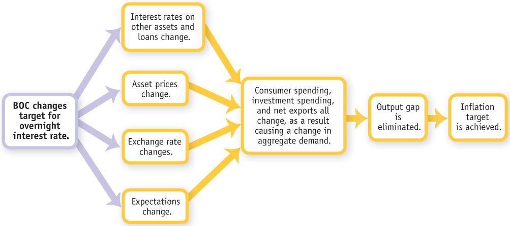
The Bank of Canada believes that changes in the target for the overnight rate can affect the Canadian economy through four different channels: interest rates on other assets and loans, asset prices, the exchange rate, and market expectations.5 Consider what happens when the economy is in a recessionary gap or in a negative output gap (where actual output is below potential output). To eliminate the recessionary gap, the Bank of Canada will lower the overnight rate target. A fall in the target for the overnight rate affects the economy via the four different channels, as follows:
Interest rates on other assets and loans There is a close link between the target for the overnight rate and interest rates on other assets in the economy, such as the prime rate and mortgage interest rates. Although there may not be a one-
Asset prices As we mentioned in Chapter 10, holding all else constant, there is an inverse relationship between interest rates and asset prices. A fall in interest rates will raise the prices of various assets such as bonds, stocks, and houses. Seeing their wealth increase when asset prices increase, households increase their spending on final goods and services (the wealth effect mentioned in Chapter 12).
The exchange rate A fall in Canadian interest rates will make Canadian assets less attractive to investors. Foreign investors will buy fewer Canadian assets, while Canadian investors will buy more foreign assets. The rise in net foreign investment (or the outflows of financial capital) that results causes the Canadian dollar to depreciate in the foreign exchange market. A weaker currency makes Canadian goods become less expensive and stimulates our net exports.
Market expectations As mentioned in Chapter 7, agents use the available information to form expectations, which they act on. When the BOC lowers the target for the overnight rate, agents would expect the inflation rate to rise in the future. Along with a higher inflation rate, they would also expect future increases in interest rates and wages, all factors that would encourage the agents to increase their spending on investment and consumption now.
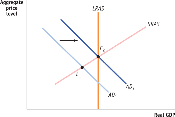
In a nutshell, if the economy finds itself in a recessionary gap, point E1 shown in Figure 15-10, then, when the BOC lowers the target for the overnight rate, this brings about an increase in the money supply, and we would expect to see an increase in consumption, investment, and net exports. These increases raise the aggregate demand for goods and services and help to eliminate a negative output (or, recessionary) gap. Later, when the economy gains momentum, the aggregate price level rises, as does the rate of inflation. This increase in the money supply shifts the aggregate demand curve toward the right, as shown in Figure 15-10. This helps close the negative output gap, moving the economy toward the long-
Now consider Figure 15-11, which presents specific data in regard to monetary policy in practice. Panel (a) compares the core inflation rate and target for the overnight rate from 1991 to 2011. Note that they tend to move together: a rise in the core inflation rate generally triggers an increase in the target for the overnight rate. It is also apparent that the BOC has succeeded in keeping the core inflation within the target range, so it can use monetary policy to tackle the output gap. Panel (b) compares, for the same years, the target for the overnight rate and the output gap (the percentage difference between actual real GDP and potential output). (Recall that the output gap is positive when actual real GDP exceeds potential output.) As you can see, the BOC tends to raise interest rates when the output gap is rising—
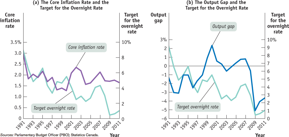
Sources: Parliamentary Budget Officer (PBO); Statistics Canada.
Inflation Targeting
Inflation targeting occurs when the central bank sets an explicit target for the inflation rate and sets monetary policy in order to hit that target.
In 1991, the Bank of Canada entered into an agreement with the federal government “to reduce inflation, as measured by the total consumer price index (CPI), from a rate of about 5 percent in late 1990 to 2 percent by the end of 1995. Inflation reached the target well ahead of schedule; and so the focus in the 1995 agreement (a renewal) shifted towards keeping it low, stable and predictable over the medium term, at an annual rate of 2 percent—
Other central banks commit themselves to achieving a specific number. For example, the Bank of England has committed to keeping inflation at 2%. In practice, there doesn’t seem to be much difference between these versions: central banks with a target range for inflation seem to aim for the middle of that range, and central banks with a fixed target and no specified upper or lower bound for acceptable inflation rates tend to give themselves considerable wiggle room.
Some economists argue that monetary policy should be based on current and past economic conditions, rather than forecasts of future conditions. They may even use formulas that determine the target interest rate as a function of the current inflation rate and output gap or the unemployment rate. In contrast to this policy of looking backward, inflation targeting looks forward. That is, inflation targeting is based on a forecast of future inflation.
Advocates of inflation targeting argue that it has two key advantages over a backward-
Critics of inflation targeting argue that it’s too restrictive because there are times when other concerns—
To achieve its inflation target, the BOC adjusts (raises or lowers) its target for the overnight interest rate, which, in turn, influences other market interest rates and the exchange rate, thereby shifting the AD curve. Changes in monetary policy take between six and eight quarters to fully work their way through the economy and have their cumulative effect on AD and inflation. This explains why the BOC sets its policy rate in a forward-
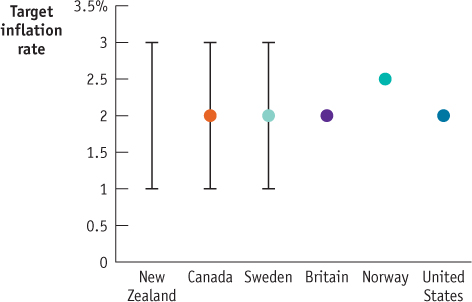
INFLATION TARGETS
This figure shows the target inflation rates of six central banks that have adopted inflation targeting. The central bank of New Zealand introduced inflation targeting in 1990. Today it has an inflation target range of 1% to 3%. The central banks of Canada and Sweden have the same target range but also specify 2% as the precise target. The central banks of Britain and Norway have specific targets for inflation, 2% and 2.5%, respectively. Neither states by how much they’re prepared to miss those targets. Since 2012, the U.S. Federal Reserve also targets inflation at 2%.
In practice, these differences in detail don’t seem to lead to any significant difference in results. New Zealand aims for the middle of its range, at 2% inflation; Britain, Norway, and the United States allow themselves considerable wiggle room around their target inflation rates.
The Zero Lower Bound Problem
Regardless of whether monetary policy is based on rules that look forward or backward, it will always face one problem: the nominal rate of interest usually has a lower bound of zero. Why? Because people always have the alternative of holding cash, which offers a zero interest rate. Normally, nobody would buy a bond yielding an interest rate less than zero because holding cash would be a better alternative.9
The fact that interest rates can’t go below zero—called the zero lower bound for interest rates—sets limits to the power of monetary policy. In 2009 and 2010, inflation was low and the U.S. economy was operating far below potential, so the U.S. Federal Reserve wanted to increase aggregate demand. Yet it could not do so in the normal way—buying short-term U.S. government debt on the open market to expand the money supply—because short-term U.S. interest rates were already at or near zero percent.
The zero lower bound for interest rates means that interest rates cannot fall below zero.
So, in November 2010, the Fed tried to solve this problem using quantitative easing. As we have already pointed out, long-term interest rates don’t follow short-term rates exactly. The short-term U.S. debt rates, for example on three-month treasury bills, were close to zero percent. But the rates for longer-term debt were higher: for example, five-year or six-year bonds were at about two or three percent. With quantitative easing (QE), the Fed began to buy longer-term U.S. government debt. The Fed hoped that buying these longer-term bonds directly would drive down interest rates on long-term debt, thus exerting an expansionary effect on the U.S. economy.
Quantitative easing (QE) is a monetary policy in which a government tries to drive down interest rates, thus exerting an expansionary effect on the economy, by buying longer-term government bonds, instead of the shorter-term bonds it would buy usually.
This policy may have given the U.S. economy some boost in 2011, but as of early 2012, recovery remained painfully slow. Over this time period, the Bank of England and the European Central Bank also used quantitative easing to try to solve England and Europe’s financial difficulties. At the same time, Canada was in a similar fix: from April 2009 to June 2010, the BOC’s target for the overnight interest rate was 0.25 percent. Unlike its counterparts, however, the BOC was not forced to try quantitative easing because our stronger financial system meant that in many ways the impact of the crisis was not as severe in Canada and our recovery was quicker.
Most economists felt that the decision to refrain from QE was a positive sign for Canada. It was a sign of Canada’s financial strength and of our economy’s recovery from the recession. Furthermore, if the Bank had tried QE, longer-term interest rates would have declined, inducing households to increase their debts, which were already at historic highs. Since Canada’s longer-term rates remained relatively high, households were induced to decrease their debt.
In contrast, some economists felt that the decision harmed our economy: QE tends to lower the value of the currencies of the countries or regions using it. Consequently, opting out of QE while many of our trading partners were engaged in it raised the value of the Canadian dollar. As a result our trade balance was harmed and jobs in export-oriented sectors of the Canadian economy were killed.
The U.S. Federal Reserve undertook three rounds of QE. The first round, in November 2008, resulted in the Fed’s assets swelling by 140% to about $2.2 trillion U.S. This first round of asset purchases helped to lower the 10-year interest rate to 2.93% at the end of November, 1 percentage point lower than the previous month. Subsequent rounds of asset purchases occurred in November 2010 and September 2012. These purchases helped to push the 10-year rate down to 1.57% at the end of September 2012. Unfortunately, even though the Fed bought a significant amount of assets in an attempt to raise the money supply and stimulate the economy, U.S. banks, rather than lending these funds out to others, responded to the fear and uncertainty by raising the amount of reserves they held on account at the Fed by more than 100%. In mid-to late 2009 the (negative) output gap was about 7.5% and the unemployment rate peaked at 10%. The U.S. economy ended 2012 with output almost 6% below potential, an unemployment rate of almost 8% (up 3 percentage points compared to January 2008), and employment still more than 3.2 million below what it had been at the start of 2008. So there is little doubt that without QE the American economy would likely have suffered more. Nonetheless the fact that multiple rounds were undertaken and that the American economy continues to suffer implies that either the degree of QE intervention was too small or that QE itself is not effective enough.
WHAT THE CENTRAL BANK WANTS, THE CENTRAL BANK GETS
What’s the evidence that a central bank can actually cause an economic contraction or expansion? You might think that it’s just a matter of seeing what happens to the economy when interest rates go up or down. But there’s a big problem with that approach: a central bank usually changes interest rates in an attempt to tame the business cycle, raising rates if the economy is expanding (and creating inflationary pressure) and reducing them if the economy is slumping (and creating low inflationary and/or deflationary pressure). So, in the actual data, it often looks as if low interest rates go along with a weak economy and high rates go along with a strong economy.
In a famous 1994 paper titled “Monetary Policy Matters,” macroeconomists Christina Romer and David Romer solved this problem by focusing on episodes in which U.S. monetary policy wasn’t a reaction to the business cycle. Specifically, they used minutes from the U.S. Federal Open Market Committee and other sources to identify episodes “in which the Federal Reserve in effect decided to attempt to create a recession to reduce inflation.” As we’ll learn in Chapter 16, rather than monetary policy just being used as a tool of macroeconomic stabilization, sometimes it is used to eliminate embedded inflation—inflation that people believe will persist into the future. In such a case, the central bank needs to create a recessionary gap—not just eliminate an inflationary gap—to wring embedded inflation out of the economy.10
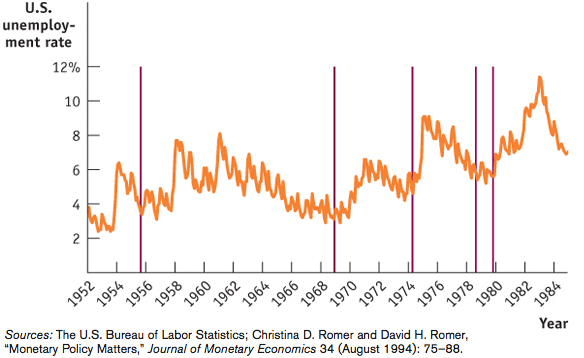
Sources: The U.S. Bureau of Labor Statistics; Christina D. Romer and David H. Romer, “Monetary Policy Matters,” Journal of Monetary Economics 34 (August 1994): 75–88.
Figure 15-12 shows the unemployment rate between 1952 and 1984 (orange) and identifies five dates on which, according to Romer and Romer, the U.S. Federal Reserve decided that it wanted a recession (vertical red lines). In four of the five cases, the decision to contract the economy was followed, after a modest lag, by a rise in the U.S. unemployment rate. On average, Romer and Romer found that the unemployment rate rises by two percentage points after the Fed decides that unemployment needs to go up.
So yes, the Fed and other central banks do get what they want.

Quick Review
The Bank of Canada can use expansionary monetary policy to increase aggregate demand and contractionary monetary policy to reduce aggregate demand. The Bank of Canada and other central banks generally try to tame the business cycle while keeping the inflation rate low but positive.
Many central banks set monetary policy by inflation targeting, a forward-looking policy rule. Although inflation targeting has the benefits of transparency and accountability, some think it is too restrictive.
Until 2008, when its target interest rate basically hit zero, the U.S. Federal Reserve’s behaviour roughly followed a backward-looking policy rule. But starting in early 2012, it began inflation targeting with a target of 2% per year.
There is a zero lower bound for interest rates—they cannot fall below zero—that limits the power of monetary policy.
In 2010, the Federal Reserve bought longer-term debt, in order to drive interest rates down and exert an expansionary effect on the economy. This policy, called quantitative easing, was also tried by the Bank of England and the European Central Bank, in each case with limited success.
Because it is subject to fewer lags than fiscal policy, monetary policy is the main tool for macroeconomic stabilization.
Check Your Understanding 15-3
CHECK YOUR UNDERSTANDING 15-3
Suppose the economy is currently suffering from an output gap and the Bank of Canada uses an expansionary monetary policy to close that gap. Describe the short-run effect of this policy on the following.
The money supply curve
The equilibrium interest rate
Investment spending
Consumer spending
Aggregate output
The money supply curve shifts to the right.
The equilibrium interest rate falls.
Investment spending rises, due to the fall in the interest rate.
Consumer spending rises, due to the multiplier process.
Aggregate output rises because of the rightward shift of the aggregate demand curve.
In setting monetary policy, which central bank—one that operates according to a backward-looking policy rule or one that operates by inflation targeting—is likely to respond more directly to a financial crisis? Explain.
The central bank that uses a backward-looking policy is likely to respond more directly to a financial crisis than one that uses inflation targeting because with a backward-looking policy the central bank does not have to set policy to meet a prespecified inflation target.