7.2 Real GDP: A Measure of Aggregate Output
In this chapter’s opening story, we described how China passed Japan as the world’s second-
The moral of this story is that the commonly cited GDP number is an interesting and useful statistic, one that provides a good way to compare the size of different economies, but it’s not a good measure of the economy’s growth over time. GDP can grow because the economy grows, but it can also grow simply because of inflation. Even if an economy’s output doesn’t change, GDP will go up if the prices of the goods and services the economy produces have increased. Likewise, GDP can fall either because the economy is producing less or because prices have fallen.
Aggregate output is the economy’s total quantity of output of final goods and services.
In order to accurately measure the economy’s growth, we need a measure of real aggregate output: the total quantity of final goods and services the economy actually produces. The measure that is used for this purpose is known as real GDP. By tracking real GDP over time, we avoid the problem of changes in prices distorting the value of changes in production of goods and services over time. Let’s look first at how real GDP is calculated, then at what it means.
Calculating Real GDP
To understand how real GDP is calculated, imagine an economy in which only two goods, apples and oranges, are produced and in which both goods are sold only to final consumers. The outputs and prices of the two fruits for two consecutive years are shown in Table 7-1.
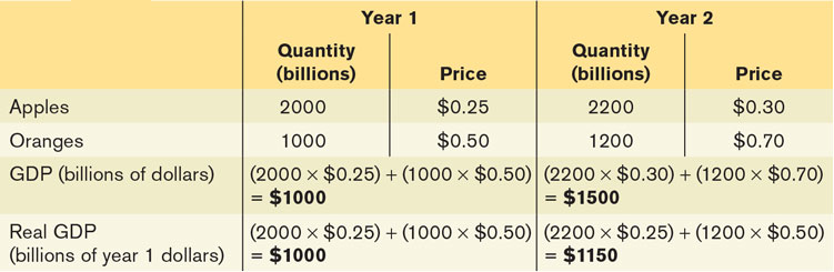
The first thing we can say about these data is that the nominal value of sales increased from year 1 to year 2. In the first year, the total value of sales was (2000 billion × $0.25) +(1000 billion × $0.50) = $1000 billion; in the second it was (2200 billion × $0.30) + (1200 billion × $0.70) = $1500 billion, which is 50% larger. But it is also clear from the table that this increase in the dollar value of GDP overstates the real growth in the economy. Although the quantities of both apples and oranges increased, the prices of both apples and oranges also rose. So part of the 50% increase in the dollar value of GDP from year 1 to year 2 simply reflects higher prices, not higher production of output.
To estimate the true increase in aggregate output produced, we have to ask the following question: how much would GDP have gone up if prices had not changed? To answer this question, we need to find the value of output in year 2 expressed in year 1 prices. In year 1 the price of apples was $0.25 each and the price of oranges $0.50 each. So year 2 output at year 1 prices is (2200 billion × $0.25) (1200 billion × $0.50) = $1150 billion. And output in year 1 at year 1 prices was $1000 billion. So in this example, GDP measured in year 1 prices rose 15%—from $1000 billion to $1150 billion.
Real GDP is the total value of all final goods and services produced in the economy during a given year, calculated using the prices of a selected base year.
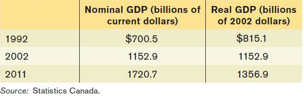
Now we can define real GDP: it is the total value of final goods and services produced in the economy during a year, calculated as if prices had stayed constant at the level of some given base year. A real GDP number always comes with information about what the base year is. Statistics Canada revises the base year every 10 years, and the current base year is 2002.
Nominal GDP is the value of all final goods and services produced in the economy during a given year, calculated using the prices (current) in the year in which the output is produced.
Sometimes, GDP is calculated using the prices of the same year in which the output is produced. Economists call this measure nominal GDP, GDP at current prices. Nominal GDP has not been adjusted for changes in prices and thus can be distorted by price changes (i.e., inflation or deflation). If we had used nominal GDP to measure the true change in output from year 1 to year 2 in our apples and oranges example, we would have overstated the true growth in output: we would have claimed it to be 50%, when in fact it was only 15%. By comparing output in the two years using the same set of prices—
Table 7-2 shows a real-
You might have noticed that there is an alternative way to calculate real GDP using the data in Table 7-1. Why not measure it using the prices of year 2 rather than year 1 as the base-
Chained dollars is the method of calculating changes in real GDP using the average between the growth rate calculated using an early base year and the growth rate calculated using a late base year.
In reality, the government economists who put together Canada’s national accounts have adopted a method to measure the change in real GDP known as chain-
The Growth Rate of Canada’s Real GDP
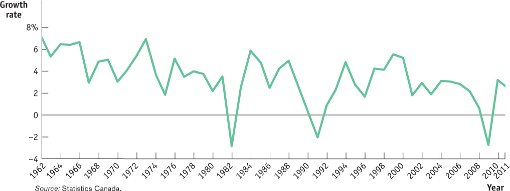
Now that we know what real GDP is, we can examine the growth rate of Canada’s real GDP. It is useful to do so, because real GDP is one of the most closely followed pieces of data that Statistics Canada releases. This is because the real GDP tells whether our economy is slowing down or expanding. Figure 7-4 depicts Canada’s real GDP growth rate from 1962 to 2011. As you see, its growth rate fluctuated during that period, showing that business cycles indeed are a common feature for any economy, including our own. As you know from Chapter 6, Canada experienced three recessions during this period: one in the early 1980s, one in the 1990s, and one in 2008–2009. The recession in the 1980s was partly the result of the two oil price shocks in the 1970s, during which the price of oil skyrocketed. The recession in the early 1990s was the result of a U.S. recession and of a deflationary (contractionary) monetary policy undertaken by the Bank of Canada. The most recent recession was triggered by the financial crises that originated in the United States. During these recessions, the country’s real GDP growth turned negative as firms, seeing the demand for their products soften, lowered their production. The diagram clearly shows another important fact—
GDP AND THE MEANING OF LIFE
“I’ve been rich and I’ve been poor,” the actress Mae West famously declared. “Believe me, rich is better.” But is the same true for countries?
This figure shows two pieces of information for a number of countries: how rich they are, as measured by GDP per capita, and how people assess their well-
Rich is better. Richer countries on average have higher well-
being than poor countries. Money matters less as you grow richer. The gain in life satisfaction as you go from GDP per capita of $5000 to $20 000 is greater than the gain as you go from $20 000 to $35 000.
Money isn’t everything. We Canadians seem to be more satisfied with our lives, even though we are poorer than Americans or Netherlanders. Japan is richer than most other nations, but by and large, quite miserable.
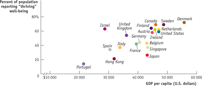
These results are consistent with the observation that high GDP per capita makes it easier to achieve a good life but that countries aren’t equally successful in taking advantage of that possibility.
Sources: Gallup; World Bank
What Real GDP Doesn’t Measure
GDP, nominal or real, is a measure of a country’s aggregate output. Other things being equal, a country with a larger population will have higher GDP simply because there are more people working. So if we want to compare GDP across countries but want to eliminate the effect of differences in population size, we use the measure GDP per capita—GDP divided by the size of the population, equivalent to the average GDP per person.
GDP per capita is GDP divided by the size of the population; it is equivalent to the average GDP per person.
Real GDP per capita can be a useful measure in some circumstances, such as in a comparison of labour productivity between countries. However, despite the fact that it is a rough measure of the average real output per person, real GDP per capita has well-known limitations as a measure of a country’s living standards. Every once in a while economists are accused of believing that growth in real GDP per capita is the only thing that matters—that is, thinking that increasing real GDP per capita is a goal in itself. In fact, economists rarely make that mistake; the idea that economists care only about real GDP per capita is a sort of urban legend. Let’s take a moment to be clear about why a country’s real GDP per capita is not a sufficient measure of human welfare in that country and why growth in real GDP per capita is not an appropriate policy goal in itself.
One way to think about this issue is to say that an increase in real GDP means an expansion in the economy’s production possibility frontier. Because the economy has increased its productive capacity, there are more things that society can achieve. But whether society actually makes good use of that increased potential to improve living standards is another matter. To put it in a slightly different way, your income may be higher this year than last year, but whether you use that higher income to actually improve your quality of life is your choice.
So let’s say it again: real GDP per capita is a measure of an economy’s average aggregate output per person—and so of what it can do. It is not a sufficient goal in itself because it doesn’t address how a country uses that output to affect living standards. A country with a high GDP can afford to be healthy, to be well educated, and in general to have a good quality of life. But there is not a one-to-one match between GDP and the quality of life.
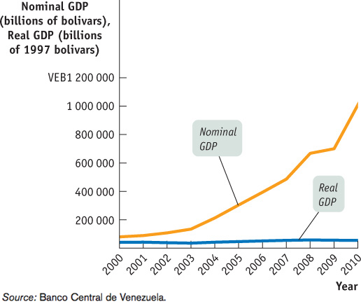
MIRACLE IN VENEZUELA?
The South American nation of Venezuela has a distinction that may surprise you: in recent years, it has had one of the world’s fastest-growing nominal GDPs. Between 2000 and 2010, Venezuelan nominal GDP grew by an average of 29% each year—much faster than nominal GDP in Canada, the United States or even in booming economies like China.
So is Venezuela experiencing an economic miracle? No, it’s just suffering from unusually high inflation. Figure 7-5 shows Venezuela’s nominal and real GDP from 2000 to 2010, with real GDP measured in 1997 prices. Real GDP did grow over the period, but at an annual rate of only 3%. This was higher than the growth rate in Canada, which was 1.7% over the same period, but it is far short of China’s 10% growth.

Quick Review
To determine the actual growth in aggregate output, we calculate real GDP using prices from some given base year. In contrast, nominal GDP is the value of aggregate output calculated with current prices. Canadian statistics on real GDP are always expressed in chained dollars.
Real GDP per capita is a measure of the average aggregate output per person. But it is not a sufficient measure of human welfare, nor is it an appropriate goal in itself, because it does not reflect important aspects of living standards within an economy.
Check Your Understanding 7-2
CHECK YOUR UNDERSTANDING 7-2
Assume there are only two goods in the economy, french fries and onion rings. In 2011, 1 000 000 servings of french fries were sold at $0.40 each and 800 000 servings of onion rings at $0.60 each. From 2011 to 2012, the price of french fries rose by 25% and the servings sold fell by 10%; the price of onion rings fell by 15% and the servings sold rose by 5%.
Calculate nominal GDP in 2011 and 2012. Calculate real GDP in 2012 using 2011 prices.
Why would an assessment of growth using nominal GDP be misguided?
In 2011 nominal GDP was (1 000 000 × $0.40) + (800 000 × $0.60) = $400 000 + $480 000 = $880 000. A 25% rise in the price of french fries from 2011 to 2012 means that the 2012 price of french fries was 1.25 × $0.40 = $0.50. A 10% fall in servings means that 1 000 000 × 0.9 = 900 000 servings were sold in 2012. As a result, the total value of sales of french fries in 2012 was 900 000 × $0.50 = $450 000. A 15% fall in the price of onion rings from 2011 to 2012 means that the 2012 price of onion rings was 0.85 × $0.60 = $0.51. A 5% rise in servings sold means that 800 000 × 1.05 = 840 000 servings were sold in 2012. As a result, the total value of sales of onion rings in 2012 was 840 000 × $0.51 = $428 400. Nominal GDP in 2012 was $450 000 + $428 400 = $878 400. To find real GDP in 2012, we must calculate the value of sales in 2012 using 2011 prices: (900 000 french fries × $0.40) + (840 000 onion rings × $0.60) = $360 000 + $504 000 = $864 000.
A comparison of nominal GDP in 2011 to nominal GDP in 2012 shows a decline of (($880 000 − $878 400)/$880 000) × 100 = 0.18%. But a comparison using real GDP shows a decline of (($880 000 – $864 000)/$880 000) × 100 = 1.8%. That is, a calculation based on real GDP shows a drop 10 times larger (1.8%) than a calculation based on nominal GDP (0.18%). In this case, the calculation based on nominal GDP underestimates the true magnitude of the change.
From 2005 to 2010, the price of electronic equipment fell dramatically and the price of housing rose dramatically. What are the implications of this in deciding whether to use 2005 or 2010 as the base year in calculating 2012 real GDP?
A price index based on 2005 prices will contain a relatively high price of electronics and a relatively low price of housing compared to a price index based on 2010 prices. This means that a 2005 price index used to calculate real GDP in 2012 will magnify the value of electronics production in the economy, but a 2010 price index will magnify the value of housing production in the economy.