Consumer Spending
Should you splurge on a restaurant meal or save money by eating at home? Should you buy a new car and, if so, how expensive a model? Should you redo that bathroom or live with it for another year? In the real world, households are constantly confronted with such choices—
But what determines how much consumers spend?
Current Disposable Income and Consumer Spending
The most important factor affecting a family’s consumer spending is its current disposable income—
The Bureau of Labor Statistics (BLS) collects annual data on family income and spending. Families are grouped by levels of before-
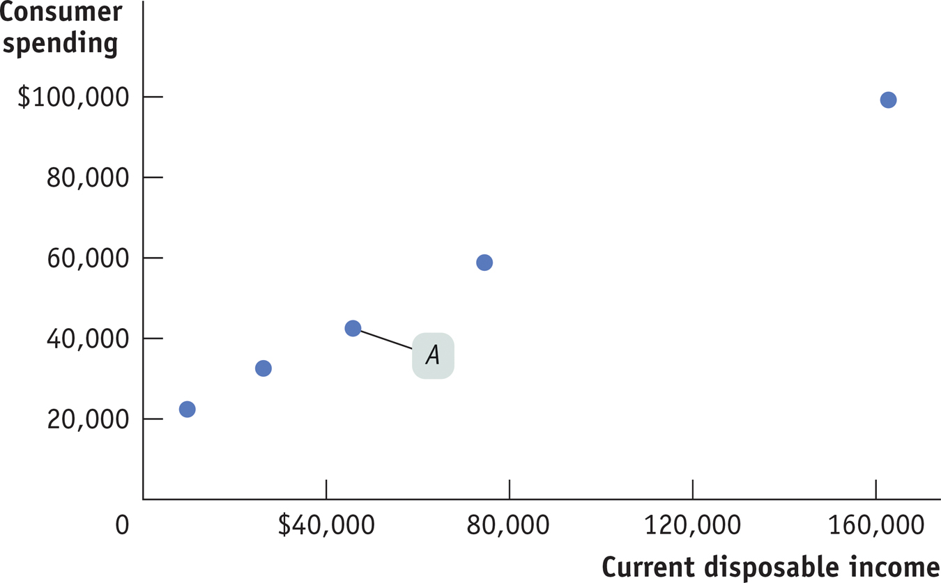
Figure 26-2 is a scatter diagram illustrating the relationship between household current disposable income and household consumer spending for American households by income group in 2013. For example, point A shows that in 2013 the middle fifth of the population had an average current disposable income of $45,826 and average spending of $42,495. The pattern of the dots slopes upward from left to right, making it clear that households with higher current disposable income had higher consumer spending.
26-2
Current Disposable Income and Consumer Spending for American Households in 2013

It’s very useful to represent the relationship between an individual household’s current disposable income and its consumer spending with an equation. The consumption function is an equation showing how an individual household’s consumer spending varies with the household’s current disposable income. The simplest version of a consumption function is a linear equation:
The consumption function is an equation showing how an individual household’s consumer spending varies with the household’s current disposable income.

where lowercase letters indicate variables measured for an individual household.
In this equation, c is individual household consumer spending and yd is individual household current disposable income. Recall that MPC, the marginal propensity to consume, is the amount by which consumer spending rises if current disposable income rises by $1. Finally, a is a constant term—
Recall that we expressed MPC as the ratio of a change in consumer spending to the change in current disposable income. We’ve rewritten it for an individual household as Equation 26-

Multiplying both sides of Equation 26-

Equation 26-
Figure 26-3 shows what Equation 26-
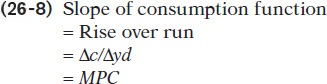
26-3
The Consumption Function
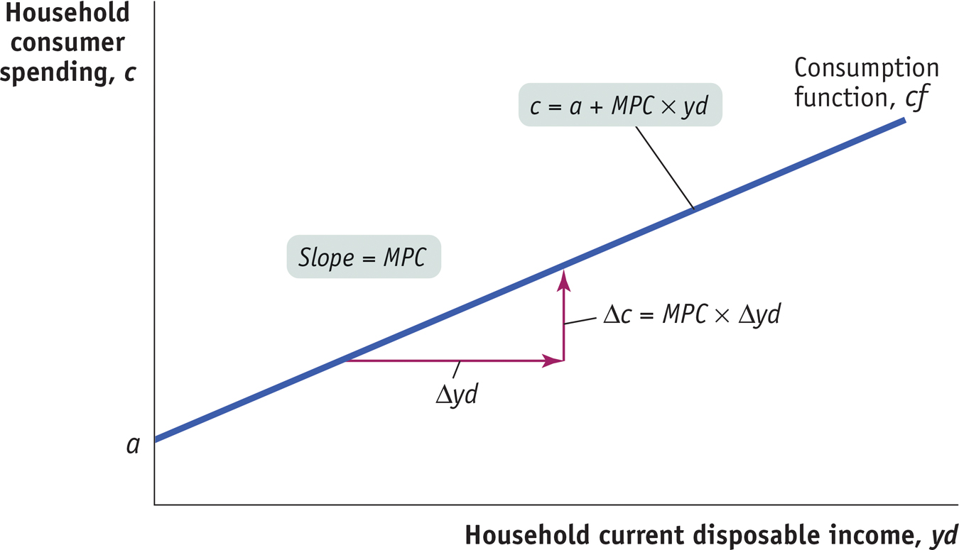
In reality, actual data never fit Equation 26-
c = $19,343 + 0.50 × yd
26-4
A Consumption Function Fitted to Data
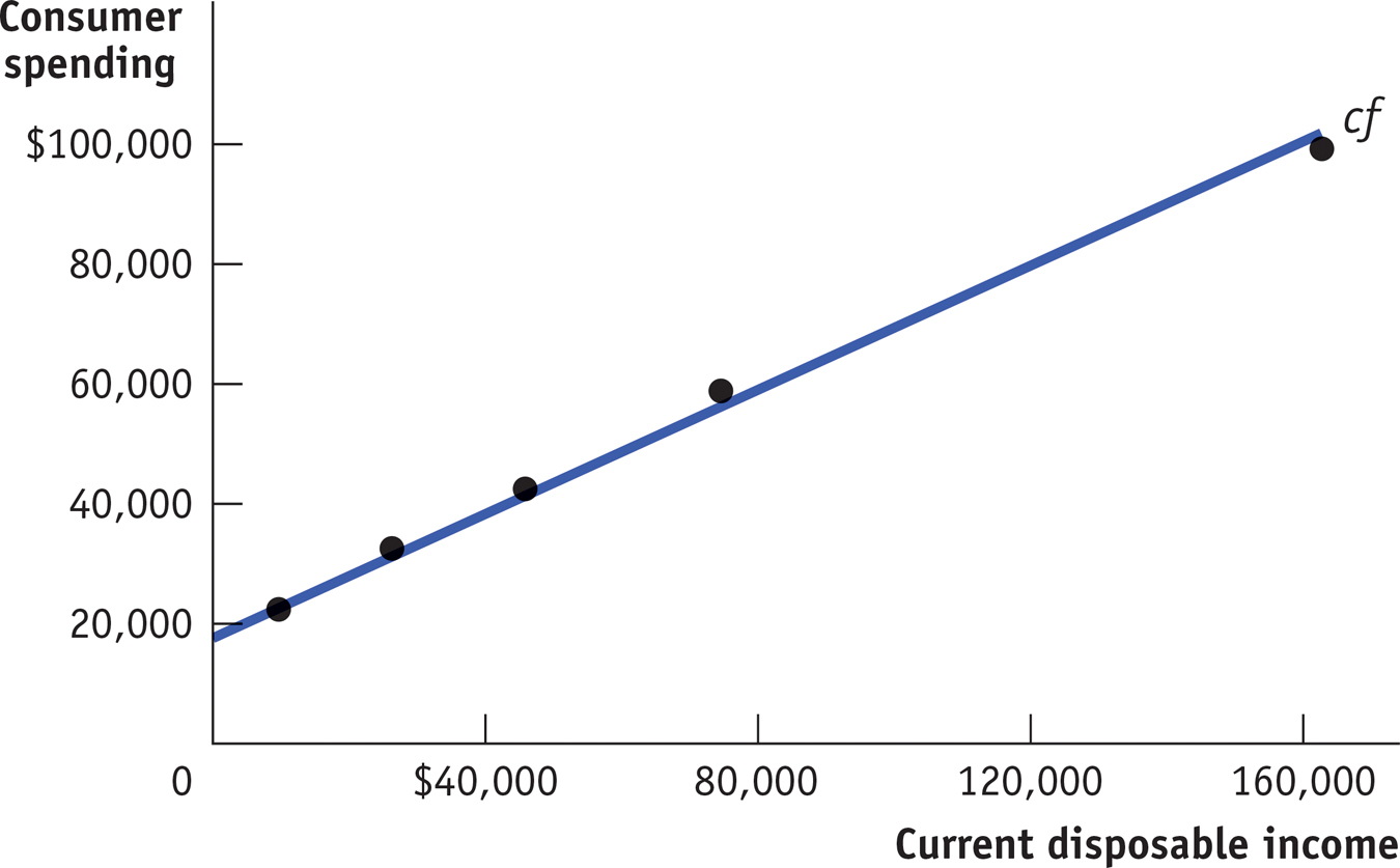
That is, the data suggest a marginal propensity to consume of approximately 0.50. This implies that the marginal propensity to save (MPS)—the amount of an additional $1 of disposable income that is saved—
It’s important to realize that Figure 26-4 shows a microeconomic relationship between the current disposable income of individual households and their spending on goods and services. However, macroeconomists assume that a similar relationship holds for the economy as a whole: that there is a relationship, called the aggregate consumption function, between aggregate current disposable income and aggregate consumer spending. We’ll assume that it has the same form as the household-
The aggregate consumption function is the relationship for the economy as a whole between aggregate current disposable income and aggregate consumer spending.

Here, C is aggregate consumer spending (called just “consumer spending”); YD is aggregate current disposable income (called, for simplicity, just “disposable income”); and A is aggregate autonomous consumer spending, the amount of consumer spending when YD equals zero. This is the relationship represented in Figure 26-5 by CF, analogous to cf in Figure 26-3.
26-5
Shifts of the Aggregate Consumption Function
Shifts of the Aggregate Consumption Function
The aggregate consumption function shows the relationship between disposable income and consumer spending for the economy as a whole, other things equal. When things other than disposable income change, the aggregate consumption function shifts. There are two principal causes of shifts of the aggregate consumption function: changes in expected future disposable income and changes in aggregate wealth.
Changes in Expected Future Disposable Income Suppose you land a really good, well-
Conversely, suppose you have a good job but learn that the company is planning to downsize your division, raising the possibility that you may lose your job and have to take a lower-
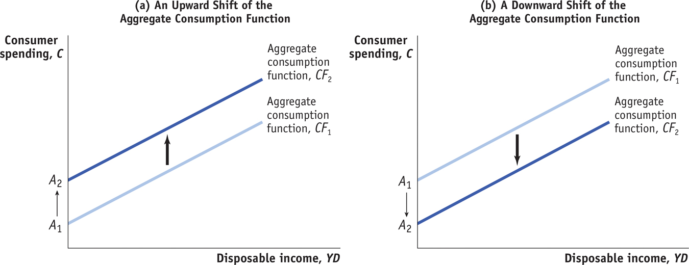
Both of these examples show how expectations about future disposable income can affect consumer spending. The two panels of Figure 26-5, which plot disposable income against consumer spending, show how changes in expected future disposable income affect the aggregate consumption function. In both panels, CF1 is the initial aggregate consumption function. Panel (a) shows the effect of good news: information that leads consumers to expect higher disposable income in the future than they did before.
Consumers will now spend more at any given level of current disposable income, YD, corresponding to an increase in A, aggregate autonomous consumer spending, from A1 to A2. The effect is to shift the aggregate consumption function up, from CF1 to CF2. Panel (b) shows the effect of bad news: information that leads consumers to expect lower disposable income in the future than they did before. Consumers will now spend less at any given level of current disposable income, YD, corresponding to a fall in A from A1 to A2. The effect is to shift the aggregate consumption function down, from CF1 to CF2.
In a famous 1956 book, A Theory of the Consumption Function, Milton Friedman showed that taking the effects of expected future income into account explains an otherwise puzzling fact about consumer behavior. If we look at consumer spending during any given year, we find that people with high current income save a larger fraction of their income than those with low current income. (This is obvious from the data in Figure 26-4: people in the highest income group spend considerably less than their income; those in the lowest income group spend more than their income.) You might think this implies that the overall savings rate will rise as the economy grows and average current incomes rise; in fact, however, this hasn’t happened.
Friedman pointed out that when we look at individual incomes in a given year, there are systematic differences between current and expected future income that create a positive relationship between current income and the savings rate. On one side, people with low current incomes are often having an unusually bad year. For example, they may be workers who have been laid off but will probably find new jobs eventually. They are people whose expected future income is higher than their current income, so it makes sense for them to have low or even negative savings. On the other side, people with high current incomes in a given year are often having an unusually good year. For example, they may have investments that happened to do extremely well. They are people whose expected future income is lower than their current income, so it makes sense for them to save most of their windfall.

When the economy grows, by contrast, current and expected future incomes rise together. Higher current income tends to lead to higher savings today, but higher expected future income tends to lead to less savings today. As a result, there’s a weaker relationship between current income and the savings rate.
Friedman argued that consumer spending ultimately depends mainly on the income people expect to have over the long term rather than on their current income. This argument is known as the permanent income hypothesis.
Changes in Aggregate Wealth Imagine two individuals, Maria and Mark, both of whom expect to earn $30,000 this year. Suppose, however, that they have different histories. Maria has been working steadily for the past 10 years, owns her own home, and has $200,000 in the bank. Mark is the same age as Maria, but he has been in and out of work, hasn’t managed to buy a house, and has very little in savings. In this case, Maria has something that Mark doesn’t have: wealth. Even though they have the same disposable income, other things equal, you’d expect Maria to spend more on consumption than Mark. That is, wealth has an effect on consumer spending.
The effect of wealth on spending is emphasized by an influential economic model of how consumers make choices about spending versus saving called the life-
Because wealth affects household consumer spending, changes in wealth across the economy can shift the aggregate consumption function. A rise in aggregate wealth—
ECONOMICS in Action: Famous First Forecasting Failures
Famous First Forecasting Failures
The Great Depression created modern macroeconomics. It also gave birth to the modern field of econometrics—
Figure 26-6 tells the story. Panel (a) shows aggregate data on disposable income and consumer spending from 1929 to 1941, measured in billions of 2005 dollars. A simple linear consumption function, CF1, seems to fit the data very well. And many economists thought this relationship would continue to hold in the future. But panel (b) shows what actually happened in later years. The points in the circle at the left are the data from the Great Depression shown in panel (a). The points in the circle at the right are data from 1946 to 1960. (Data from 1942 to 1945 aren’t included because rationing during World War II prevented consumers from spending normally.) The solid line in the figure, CF1, is the consumption function fitted to 1929–
26-6
Changes in the Aggregate Consumption Function Over Time
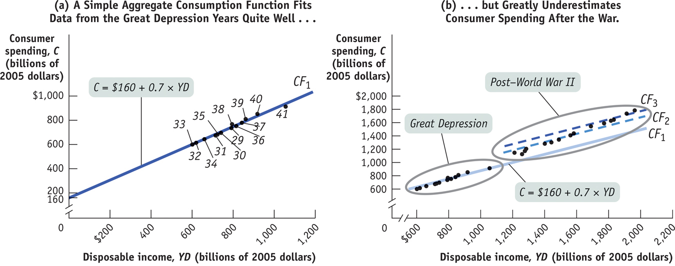
Why was extrapolating from the earlier relationship so misleading? The answer is that from 1946 onward, both expected future disposable income and aggregate wealth were steadily rising. Consumers grew increasingly confident that the Great Depression wouldn’t reemerge and that the post–
In macroeconomics, failure—
Quick Review
The consumption function shows the relationship between an individual household’s current disposable income and its consumer spending.
The aggregate consumption function shows the relationship between disposable income and consumer spending across the economy. It can shift due to changes in expected future disposable income and changes in aggregate wealth.
26-2
Question 11.4
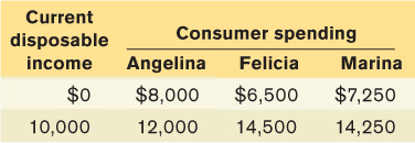
Suppose the economy consists of three people: Angelina, Felicia, and Marina. The table shows how their consumer spending varies as their current disposable income rises by $10,000.
Derive each individual’s consumption function, where MPC is calculated for a $10,000 change in current disposable income.
Angelina’s autonomous consumer spending is $8,000. When her current disposable income rises by $10,000, her consumer spending rises by $12,000 − $8,000 = $4,000. So her MPC is $4,000/$10,000 = 0.4 and her consumption function is c = $8,000 + 0.4 × yd. Felicia’s autonomous consumer spending is $6,500. When her current disposable income rises by $10,000, her consumer spending rises by $14,500 − $6,500 = $8,000. So her MPC is $8,000/$10,000 = 0.8 and her consumption function is c = $6,500 + 0.8 × yd. Marina’s autonomous consumer spending is $7,250. When her current disposable income rises by $10,000, her consumer spending rises by $14,250 − $7,250 = $7,000. So her MPC is $7,000/$10,000 = 0.7 and her consumption function is c = $7,250 + 0.7 × yd.
Derive the aggregate consumption function.
The aggregate autonomous consumer spending in this economy is $8,000 + $6,500 + $7,250 = $21,750. A $30,000 increase in disposable income (3 × $10,000) leads to a $4,000 + $8,000 + $7,000 = $19,000 increase in consumer spending. So the economy-wide MPC is $19,000/$30,000 = 0.63 and the aggregate consumption function is C = $21,750 + 0.63 × YD.
Question 11.5
Suppose that problems in the capital markets make consumers unable either to borrow or to put money aside for future use. What implication does this have for the effects of expected future disposable income on consumer spending?
If you expect your future disposable income to fall, you would like to save some of today’s disposable income to tide you over in the future. But you cannot do this if you cannot save. If you expect your future disposable income to rise, you would like to spend some of tomorrow’s higher income today. But you cannot do this if you cannot borrow. If you cannot save or borrow, your expected future disposable income will have no effect on your consumer spending today. In fact, your MPC must always equal 1: you must consume all your current disposable income today, and you will be unable to smooth your consumption over time.
Solutions appear at back of book.