Fiscal Policy and the Multiplier
An expansionary fiscal policy, like the 2009 U.S. stimulus, pushes the aggregate demand curve to the right. A contractionary fiscal policy, like Lyndon Johnson’s tax surcharge, pushes the aggregate demand curve to the left. For policy makers, however, knowing the direction of the shift isn’t enough: they need estimates of how much a given policy will shift the aggregate demand curve. To get these estimates, they use the concept of the multiplier, which we learned about in Chapter 26.
Multiplier Effects of an Increase in Government Purchases of Goods and Services
Suppose that a government decides to spend $50 billion building bridges and roads. The government’s purchases of goods and services will directly increase total spending on final goods and services by $50 billion. But as we learned in Chapter 26, there will also be an indirect effect: the government’s purchases will start a chain reaction throughout the economy. The firms that produce the goods and services purchased by the government earn revenues that flow to households in the form of wages, profits, interest, and rent. This increase in disposable income leads to a rise in consumer spending. The rise in consumer spending, in turn, induces firms to increase output, leading to a further rise in disposable income, which leads to another round of consumer spending increases, and so on.
As we know, the multiplier is the ratio of the change in real GDP caused by an autonomous change in aggregate spending to the size of that autonomous change. An increase in government purchases of goods and services is a prime example of such an autonomous increase in aggregate spending.
In Chapter 26 we considered a simple case in which there are no taxes or international trade, so that any change in GDP accrues entirely to households. We also assumed that the aggregate price level is fixed, so that any increase in nominal GDP is also a rise in real GDP, and that the interest rate is fixed. In that case the multiplier is 1/(1 − MPC). Recall that MPC is the marginal propensity to consume, the fraction of an additional dollar in disposable income that is spent. For example, if the marginal propensity to consume is 0.5, the multiplier is 1/(1 − 0.5) = 1/0.5 = 2. Given a multiplier of 2, a $50 billion increase in government purchases of goods and services would increase real GDP by $100 billion. Of that $100 billion, $50 billion is the initial effect from the increase in G, and the remaining $50 billion is the subsequent effect arising from the increase in consumer spending.
What happens if government purchases of goods and services are instead reduced? The math is exactly the same, except that there’s a minus sign in front: if government purchases of goods and services fall by $50 billion and the marginal propensity to consume is 0.5, real GDP falls by $100 billion.
Multiplier Effects of Changes in Government Transfers and Taxes
Expansionary or contractionary fiscal policy need not take the form of changes in government purchases of goods and services. Governments can also change transfer payments or taxes. In general, however, a change in government transfers or taxes shifts the aggregate demand curve by less than an equal-

To see why, imagine that instead of spending $50 billion on building bridges, the government simply hands out $50 billion in the form of government transfers. In this case, there is no direct effect on aggregate demand, as there was with government purchases of goods and services. Real GDP goes up only because households spend some of that $50 billion—
Table 28-1 shows a hypothetical comparison of two expansionary fiscal policies assuming an MPC equal to 0.5 and a multiplier equal to 2: one in which the government directly purchases $50 billion in goods and services and one in which the government makes transfer payments instead, sending out $50 billion in checks to consumers. In each case there is a first-
28-1
Hypothetical Effects of a Fiscal Policy with Multiplier of 2
|
Effect on real GDP |
$50 billion rise in government purchases of goods and services |
$50 billion rise in government transfer payments |
|---|---|---|
|
First round |
$50 billion |
$25 billion |
|
Second round |
$25 billion |
$12.5 billion |
|
Third round |
$12.5 billion |
$6.25 billion |
|
• |
• |
• |
|
• |
• |
• |
|
• |
• |
• |
|
Eventual effect |
$100 billion |
$50 billion |
TABLE 13-
However, the first-
Overall, when expansionary fiscal policy takes the form of a rise in transfer payments, real GDP may rise by either more or less than the initial government outlay—
A tax cut has an effect similar to the effect of a transfer. It increases disposable income, leading to a series of increases in consumer spending. But the overall effect is smaller than that of an equal-
Lump-
We should also note that taxes introduce a further complication—
In practice, economists often argue that the size of the multiplier determines who among the population should get tax cuts or increases in government transfers. For example, compare the effects of an increase in unemployment benefits with a cut in taxes on profits distributed to shareholders as dividends. Consumer surveys suggest that the average unemployed worker will spend a higher share of any increase in his or her disposable income than would the average recipient of dividend income. That is, people who are unemployed tend to have a higher MPC than people who own a lot of stocks because the latter tend to be wealthier and tend to save more of any increase in disposable income. If that’s true, a dollar spent on unemployment benefits increases aggregate demand more than a dollar’s worth of dividend tax cuts.
How Taxes Affect the Multiplier
When we introduced the analysis of the multiplier in Chapter 26, we simplified matters by assuming that a $1 increase in real GDP raises disposable income by $1. In fact, however, government taxes capture some part of the increase in real GDP that occurs in each round of the multiplier process, since most government taxes depend positively on real GDP. As a result, disposable income increases by considerably less than $1 once we include taxes in the model.
The increase in government tax revenue when real GDP rises isn’t the result of a deliberate decision or action by the government. It’s a consequence of the way the tax laws are written, which causes most sources of government revenue to increase automatically when real GDP goes up. For example, income tax receipts increase when real GDP rises because the amount each individual owes in taxes depends positively on his or her income, and households’ taxable income rises when real GDP rises. Sales tax receipts increase when real GDP rises because people with more income spend more on goods and services. And corporate profit tax receipts increase when real GDP rises because profits increase when the economy expands.
The effect of these automatic increases in tax revenue is to reduce the size of the multiplier. Remember, the multiplier is the result of a chain reaction in which higher real GDP leads to higher disposable income, which leads to higher consumer spending, which leads to further increases in real GDP. The fact that the government siphons off some of any increase in real GDP means that at each stage of this process, the increase in consumer spending is smaller than it would be if taxes weren’t part of the picture. The result is to reduce the multiplier. The appendix to this chapter shows how to derive the multiplier when taxes that depend positively on real GDP are taken into account.
Many macroeconomists believe it’s a good thing that in real life taxes reduce the multiplier. In Chapter 27 we argued that most, though not all, recessions are the result of negative demand shocks. The same mechanism that causes tax revenue to increase when the economy expands causes it to decrease when the economy contracts. Since tax receipts decrease when real GDP falls, the effects of these negative demand shocks are smaller than they would be if there were no taxes. The decrease in tax revenue reduces the adverse effect of the initial fall in aggregate demand.
Automatic stabilizers are government spending and taxation rules that cause fiscal policy to be automatically expansionary when the economy contracts and automatically contractionary when the economy expands.
The automatic decrease in government tax revenue generated by a fall in real GDP—

The rules that govern tax collection aren’t the only automatic stabilizers, although they are the most important ones. Some types of government transfers also play a stabilizing role. For example, more people receive unemployment insurance when the economy is depressed than when it is booming. The same is true of Medicaid and food stamps. So transfer payments tend to rise when the economy is contracting and fall when the economy is expanding. Like changes in tax revenue, these automatic changes in transfers tend to reduce the size of the multiplier because the total change in disposable income that results from a given rise or fall in real GDP is smaller.
As in the case of government tax revenue, many macroeconomists believe that it’s a good thing that government transfers reduce the multiplier. Expansionary and contractionary fiscal policies that are the result of automatic stabilizers are widely considered helpful to macroeconomic stabilization because they blunt the extremes of the business cycle.
Discretionary fiscal policy is fiscal policy that is the result of deliberate actions by policy makers rather than rules.
But what about fiscal policy that isn’t the result of automatic stabilizers? Discretionary fiscal policy is fiscal policy that is the direct result of deliberate actions by policy makers rather than automatic adjustment. For example, during a recession, the government may pass legislation that cuts taxes and increases government spending in order to stimulate the economy. In general, economists tend to support the use of discretionary fiscal policy only in special circumstances, such as an especially severe recession. We’ll explain why, and describe the debates among macroeconomists on the appropriate role of fiscal policy, in Chapter 33.
!worldview! ECONOMICS in Action: Austerity and the Multiplier
Austerity and the Multiplier
We’ve explained the logic of the fiscal multiplier, but what empirical evidence do economists have about multiplier effects in practice? Until a few years ago, the answer would have been that we didn’t have nearly as much evidence as we’d like.
28-7
The Fiscal Multiplier, 2009–
The problem was that large changes in fiscal policy are fairly rare, and usually happen at the same time other things are taking place, making it hard to separate the effects of spending and taxes from those of other factors. For example, the U.S. drastically increased spending during World War II—
Recent events have, however, offered considerable new evidence. As we explain later in this chapter, after 2009 several European countries found themselves facing debt crises, so they were forced to turn to the rest of Europe for aid. A condition of this aid was austerity—sharp cuts in spending plus tax increases. (We will explain austerity more fully in Chapter 32.) By comparing the economic performance of countries that were forced into austerity with that of countries that weren’t, we get a relatively clear view of the effects of changes in spending and taxes.
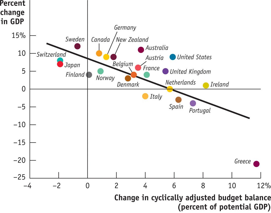
Figure 28-7 compares the amount of austerity imposed in a number of countries between 2009 and 2013 with the growth in their GDP over the same period. Austerity is measured by the change in the cyclically adjusted budget balance, defined later in this chapter. Greece—
As you might expect, economists have offered a number of qualifications and caveats to this result, coming from the fact that this wasn’t truly a controlled experiment. Overall, however, recent experience seems to support the notion that fiscal policy does indeed move GDP in the predicted direction, with a multiplier of more than 1.
Quick Review
The amount by which changes in government purchases raise real GDP is determined by the multiplier.
Changes in taxes and government transfers also move real GDP, but by less than equal-
sized changes in government purchases. Taxes reduce the size of the multiplier unless they are lump-
sum taxes .Taxes and some government transfers act as automatic stabilizers as tax revenue responds positively to changes in real GDP and some government transfers respond negatively to changes in real GDP. Many economists believe that it is a good thing that they reduce the size of the multiplier. In contrast, the use of discretionary fiscal policy is more controversial.
28-2
Question 13.4
Explain why a $500 million increase in government purchases of goods and services will generate a larger rise in real GDP than a $500 million increase in government transfers.
A $500 million increase in government purchases of goods and services directly increases aggregate spending by $500 million, which then starts the multiplier in motion. It will increase real GDP by $500 million × 1/(1 − MPC). A $500 million increase in government transfers increases aggregate spending only to the extent that it leads to an increase in consumer spending. Consumer spending rises by MPC × $1 for every $1 increase in disposable income, where MPC is less than 1. So a $500 million increase in government transfers will cause a rise in real GDP only MPC times as much as a $500 million increase in government purchases of goods and services. It will increase real GDP by $500 million × MPC/(1 − MPC).
Question 13.5
Explain why a $500 million reduction in government purchases of goods and services will generate a larger fall in real GDP than a $500 million reduction in government transfers.
This is the same issue as in Problem 1, but in reverse. If government purchases of goods and services fall by $500 million, the initial fall in aggregate spending is $500 million. If there is a $500 million reduction in government transfers, the initial fall in aggregate spending is MPC × $500 million, which is less than $500 million.
Question 13.6
The country of Boldovia has no unemployment insurance benefits and a tax system using only lump-
sum taxes. The neighboring country of Moldovia has generous unemployment benefits and a tax system in which residents must pay a percentage of their income. Which country will experience greater variation in real GDP in response to demand shocks, positive and negative? Explain. Boldovia will experience greater variation in its real GDP than Moldovia because Moldovia has automatic stabilizers while Boldovia does not. In Moldovia the effects of slumps will be lessened by unemployment insurance benefits that will support residents’ incomes, while the effects of booms will be diminished because tax revenues will go up. In contrast, incomes will not be supported in Boldovia during slumps because there is no unemployment insurance. In addition, because Boldovia has lump-sum taxes, its booms will not be diminished by increases in tax revenue.
Solutions appear at back of book.