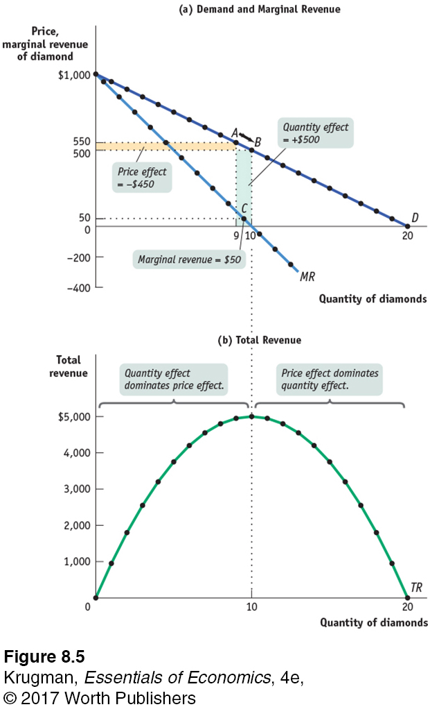Panel (a) shows the monopolist’s demand and marginal revenue curves for diamonds from Table 8-1. The marginal revenue curve lies below the demand curve. To see why, consider point A on the demand curve, where 9 diamonds are sold at $550 each, generating total revenue of $4,950. To sell a 10th diamond, the price on all 10 diamonds must be cut to $500, as shown by point B. As a result, total revenue increases by the green area (the quantity effect: + $500) but decreases by the yellow area (the price effect: −$450). So the marginal revenue from the 10th diamond is $50 (the difference between the green and yellow areas), which is much lower than its price, $500. Panel (b) shows the monopolist’s total revenue curve for diamonds. As output goes from 0 to 10 diamonds, total revenue increases. It reaches its maximum at 10 diamonds—the level at which marginal revenue is equal to 0—and declines thereafter. The quantity effect dominates the price effect when total revenue is rising; the price effect dominates the quantity effect when total revenue is falling.