19.4 Monetary Policy and Aggregate Demand
In Chapter 17 we saw how fiscal policy can be used to stabilize the economy. Now we will see how monetary policy—
Expansionary and Contractionary Monetary Policy
In Chapter 16 we learned that monetary policy shifts the aggregate demand curve. We can now explain how that works: through the effect of monetary policy on the interest rate.
Expansionary monetary policy is monetary policy that increases aggregate demand.
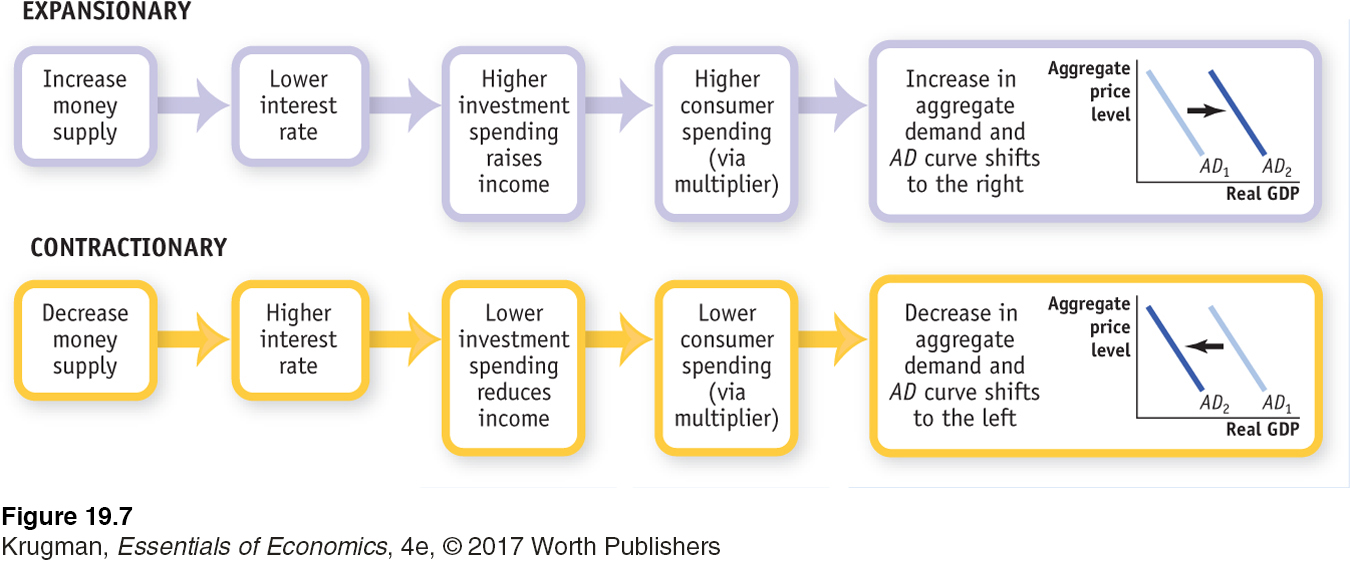
Figure 19-7 illustrates the process. Suppose, first, that the Federal Reserve wants to reduce interest rates, so it expands the money supply. As you can see in the top portion of the figure, a lower interest rate, in turn, will lead, other things equal, to more investment spending. This will in turn lead to higher consumer spending, through the multiplier process, and to an increase in aggregate output demanded. In the end, the total quantity of goods and services demanded at any given aggregate price level rises when the quantity of money increases, and the AD curve shifts to the right. Monetary policy that increases the demand for goods and services is known as expansionary monetary policy.
Contractionary monetary policy is monetary policy that decreases aggregate demand.
Suppose, alternatively, that the Federal Reserve wants to increase interest rates, so it contracts the money supply. You can see this process illustrated in the bottom portion of the diagram. Contraction of the money supply leads to a higher interest rate. The higher interest rate leads to lower investment spending, then to lower consumer spending, and then to a decrease in aggregate output demanded. So the total quantity of goods and services demanded falls when the money supply is reduced, and the AD curve shifts to the left. Monetary policy that decreases the demand for goods and services is called contractionary monetary policy.
Monetary Policy in Practice
How does the Fed decide whether to use expansionary or contractionary monetary policy? And how does it decide how much is enough? Recall that policy makers try to fight recessions, as well as try to ensure price stability: low (though usually not zero) inflation. Actual monetary policy reflects a combination of these goals.
In general, the Federal Reserve and other central banks tend to engage in expansionary monetary policy when actual real GDP is below potential output. Panel (a) of Figure 19-8 shows the U.S. output gap, which we defined in Chapter 16 as the percentage difference between actual real GDP and potential output, versus the federal funds rate since 1985. (Recall that the output gap is positive when actual real GDP exceeds potential output.) As you can see, the Fed has tended to raise interest rates when the output gap is rising—
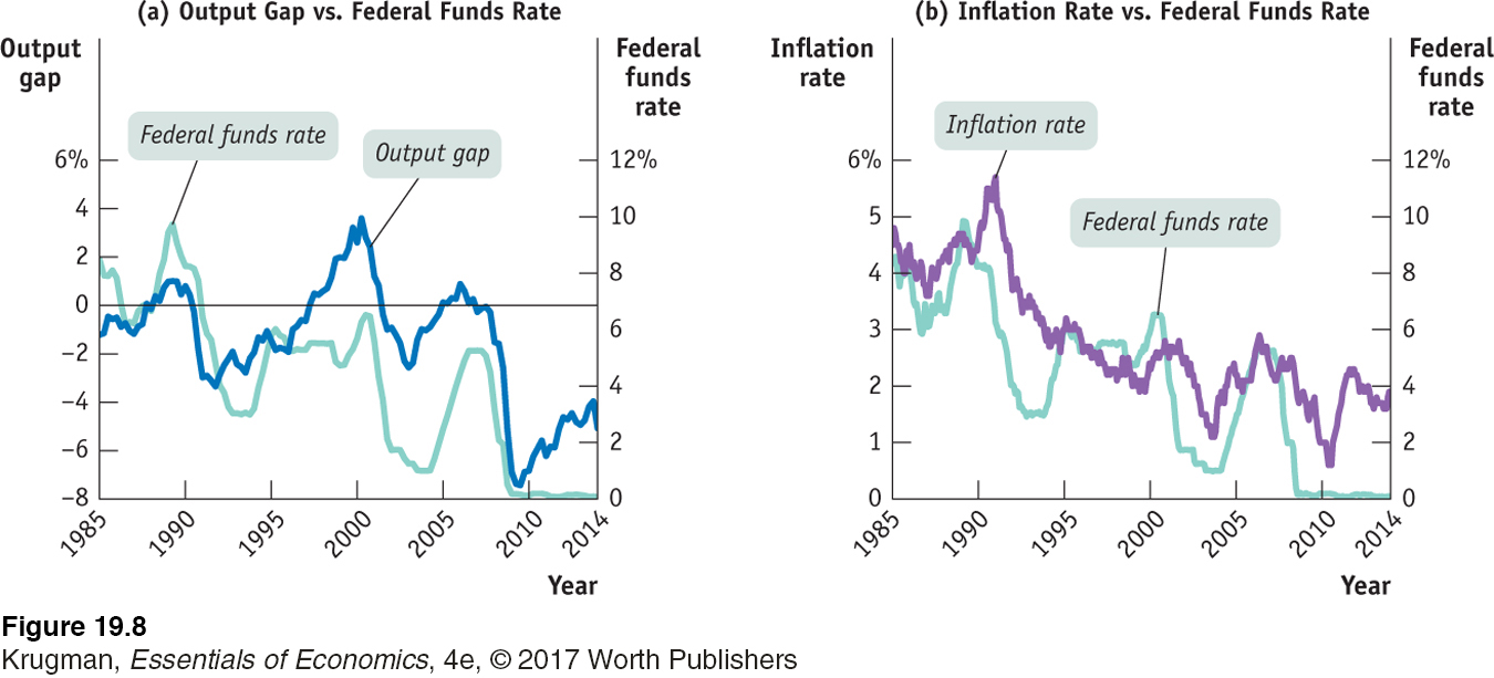
The big exception was the late 1990s, when the Fed left rates steady for several years even as the economy developed a positive output gap (which went along with a low unemployment rate). One reason the Fed was willing to keep interest rates low in the late 1990s was that inflation was low.
Panel (b) of Figure 19-8 compares the inflation rate, measured as the rate of change in consumer prices excluding food and energy, with the federal funds rate. You can see how low inflation during the mid-
The Taylor Rule Method of Setting Monetary Policy
A Taylor rule for monetary policy is a rule that sets the federal funds rate according to the level of the inflation rate and either the output gap or the unemployment rate.
In 1993 Stanford economist John Taylor suggested that monetary policy should follow a simple rule that takes into account concerns about both the business cycle and inflation. He also suggested that actual monetary policy often looks as if the Federal Reserve was, in fact, more or less following the proposed rule. A Taylor rule for monetary policy is a rule for setting interest rates that takes into account the inflation rate and the output gap or, in some cases, the unemployment rate.
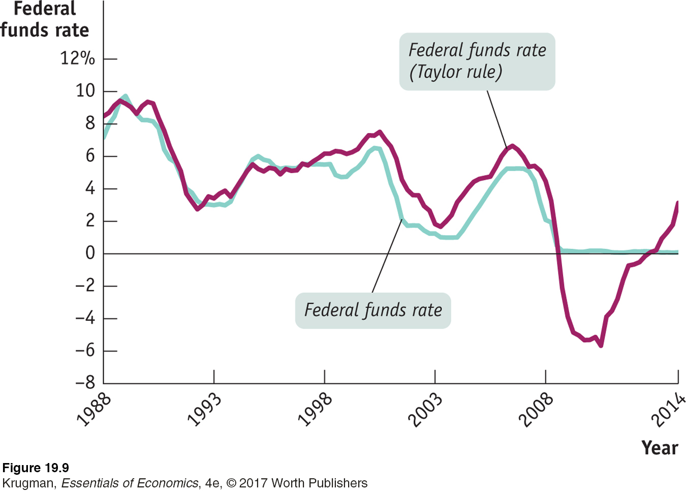
A widely cited example of a Taylor rule is a relationship among Fed policy, inflation, and unemployment estimated by economists at the Federal Reserve Bank of San Francisco. These economists found that between 1988 and 2008 the Fed’s behavior was well summarized by the following Taylor rule:
Federal funds rate = 2.07 + 1.28 × inflation rate − 1.95 × unemployment gap
where the inflation rate was measured by the change over the previous year in consumer prices excluding food and energy, and the unemployment gap was the difference between the actual unemployment rate and Congressional Budget Office estimates of the natural rate of unemployment.
Figure 19-9 compares the federal funds rate predicted by this rule with the actual federal funds rate from 1985 to mid-
Inflation Targeting
Inflation targeting occurs when the central bank sets an explicit target for the inflation rate and sets monetary policy in order to hit that target.
Until January 2012, the Fed did not explicitly commit itself to achieving a particular inflation rate. However, in January 2012, the Fed announced that it would set its policy to maintain an approximately 2% inflation rate per year. With that statement, the Fed joined a number of other central banks that have explicit inflation targets. So rather than using a Taylor rule to set monetary policy, they instead announce the inflation rate that they want to achieve—
Other central banks commit themselves to achieving a specific number. For example, the Bank of England has committed to keeping inflation at 2%. In practice, there doesn’t seem to be much difference between these versions: central banks with a target range for inflation seem to aim for the middle of that range, and central banks with a fixed target tend to give themselves considerable wiggle room.
One major difference between inflation targeting and the Taylor rule method is that inflation targeting is forward-
Advocates of inflation targeting argue that it has two key advantages over a Taylor rule: transparency and accountability. First, economic uncertainty is reduced because the central bank’s plan is transparent: the public knows the objective of an inflation-
GLOBALCOMPARISION
Inflation Targets
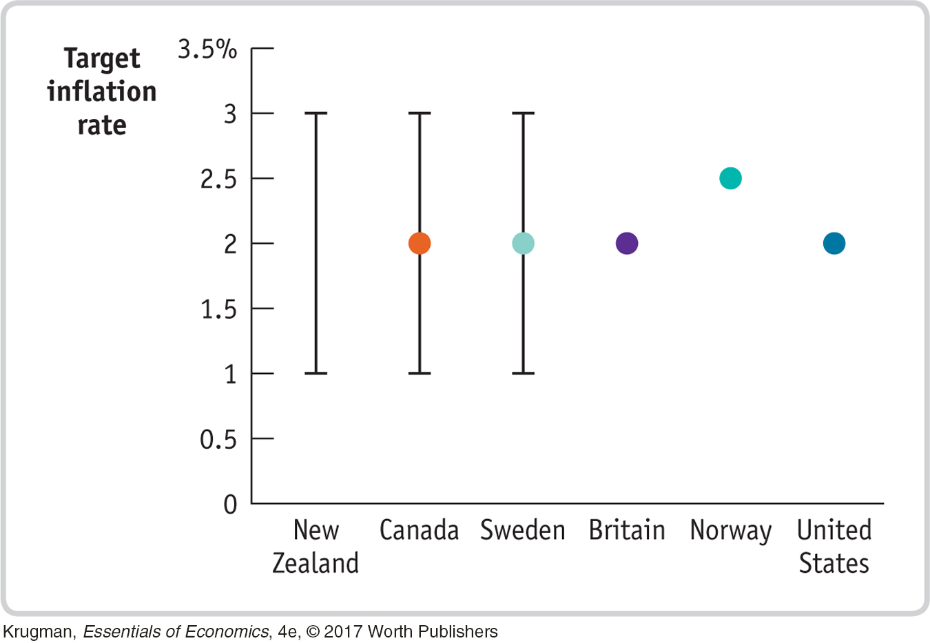
This figure shows the target inflation rates of six central banks that have adopted inflation targeting. The central bank of New Zealand introduced inflation targeting in 1990. Today it has an inflation target range of from 1% to 3%. The central banks of Canada and Sweden have the same target range but also specify 2% as the precise target. The central banks of Britain and Norway have specific targets for inflation, 2% and 2.5%, respectively. Neither states by how much they’re prepared to miss those targets. Since 2012, the U.S. Federal Reserve also targets inflation at 2%.
In practice, these differences in detail don’t seem to lead to any significant difference in results. New Zealand aims for the middle of its range, at 2% inflation; Britain, Norway, and the United States allow themselves considerable wiggle room around their target inflation rates.
Critics of inflation targeting argue that it’s too restrictive because there are times when other concerns—
Many American macroeconomists have had positive things to say about inflation targeting—
The Zero Lower Bound Problem
As Figure 19-9 shows, a Taylor rule based on inflation and the unemployment rate does a good job of predicting Federal Reserve policy from 1988 through 2008. After that, however, things go awry, and for a simple reason: with very high unemployment and low inflation, the same Taylor rule called for an interest rate less than zero, which isn’t possible.
Why aren’t negative interest rates possible? Because people always have the alternative of holding cash, which offers a zero interest rate. Nobody would ever buy a bond yielding an interest rate less than zero because holding cash would be a better alternative.
The zero lower bound for interest rates means that interest rates cannot fall below zero.
The fact that interest rates can’t go below zero—
In November 2010 the Fed began an attempt to circumvent this problem, through quantitative easing. Instead of purchasing only short-
Later the Fed expanded the program to include purchasing mortgage-
Was this policy effective? The Federal Reserve believes that it helped the economy. However, the pace of recovery remained disappointingly slow.
ECONOMICSin Action
What the Fed Wants, the Fed Gets
![]() | interactive activity
| interactive activity
What’s the evidence that the Fed can actually cause an economic contraction or expansion? You might think that finding such evidence is just a matter of looking at what happens to the economy when interest rates go up or down. But it turns out that there’s a big problem with that approach: the Fed usually changes interest rates in an attempt to tame the business cycle, raising rates if the economy is expanding and reducing rates if the economy is slumping. So in the actual data, it often looks as if low interest rates go along with a weak economy and high rates go along with a strong economy.
In a famous 1994 paper titled “Monetary Policy Matters,” the macroeconomists Christina Romer and David Romer solved this problem by focusing on episodes in which monetary policy wasn’t a reaction to the business cycle. Specifically, they used minutes from the Federal Open Market Committee and other sources to identify episodes “in which the Federal Reserve in effect decided to attempt to create a recession to reduce inflation.”
Figure 19-10 shows the unemployment rate between 1952 and 1984 and also identifies five dates on which, according to Romer and Romer, the Fed decided that it wanted a recession (the vertical lines). In four out of the five cases, the decision to contract the economy was followed, after a modest lag, by a rise in the unemployment rate. On average, Romer and Romer found, the unemployment rate rises by 2 percentage points after the Fed decides that unemployment needs to go up.
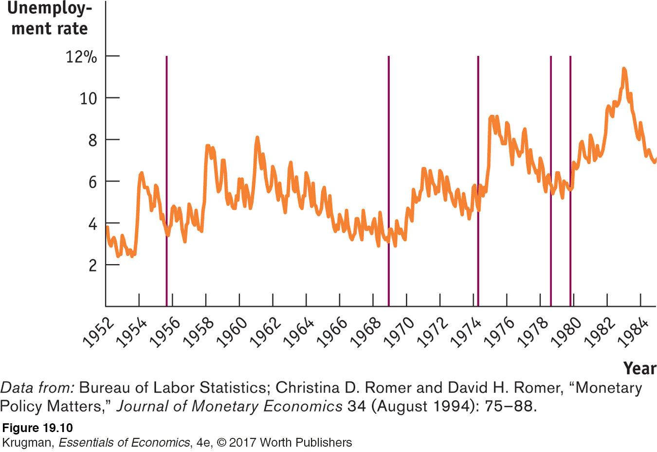
So yes, the Fed gets what it wants.
Quick Review
The Federal Reserve can use expansionary monetary policy to increase aggregate demand and contractionary monetary policy to reduce aggregate demand. The Federal Reserve and other central banks generally try to tame the business cycle while keeping the inflation rate low but positive.
Under a Taylor rule for monetary policy, the target federal funds rate rises when there is high inflation and either a positive output gap or very low unemployment; it falls when there is low or negative inflation and either a negative output gap or high unemployment.
In contrast, some central banks set monetary policy by inflation targeting, a forward-
looking policy rule, rather than by using the Taylor rule, a backward- looking policy rule. Although inflation targeting has the benefits of transparency and accountability, some think it is too restrictive. Until 2008, the Fed followed a loosely defined Taylor rule. Starting in early 2012, it began inflation targeting with a target of 2% per year. There is a zero lower bound for interest rates—
they cannot fall below zero— that limits the power of monetary policy. Because it is subject to fewer lags than fiscal policy, monetary policy is the main tool for macroeconomic stabilization.
Check Your Understanding19-3
Question 19.6
1. Suppose the economy is currently suffering from an output gap and the Federal Reserve uses an expansionary monetary policy to close that gap. Describe the short-
The money supply curve
The money supply curve shifts to the right.
The equilibrium interest rate
The equilibrium interest rate falls.
Investment spending
Investment spending rises, due to the fall in the interest rate.
Consumer spending
Consumer spending rises, due to the multiplier process.
Aggregate output
Aggregate output rises because of the rightward shift of the aggregate demand curve.
Question 19.7
2. In setting monetary policy, which central bank—
The central bank that uses a Taylor rule is likely to respond more directly to a financial crisis than one that uses inflation targeting because with a Taylor rule the central bank does not have to set policy to meet a prespecified inflation target.
Solutions appear at back of book.