20.2 Supply, Demand, and International Trade
Simple models of comparative advantage are helpful for understanding the fundamental causes of international trade. However, to analyze the effects of international trade at a more detailed level and to understand trade policy, it helps to return to the supply and demand model. We’ll start by looking at the effects of imports on domestic producers and consumers, then turn to the effects of exports.
The Effects of Imports
Figure 20-5 shows the U.S. market for phones, ignoring international trade for a moment. It introduces a few new concepts: the domestic demand curve, the domestic supply curve, and the domestic or autarky price.
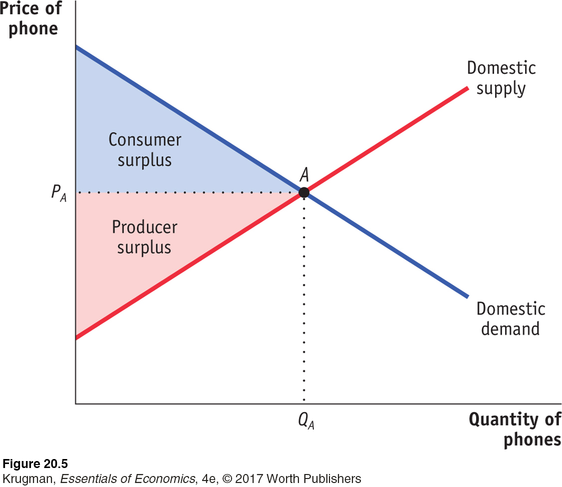
The domestic demand curve shows how the quantity of a good demanded by domestic consumers depends on the price of that good.
The domestic demand curve shows how the quantity of a good demanded by residents of a country depends on the price of that good. Why “domestic”? Because people living in other countries may demand the good, too. Once we introduce international trade, we need to distinguish between purchases of a good by domestic consumers and purchases by foreign consumers. So the domestic demand curve reflects only the demand of residents of our own country.
The domestic supply curve shows how the quantity of a good supplied by domestic producers depends on the price of that good.
Similarly, the domestic supply curve shows how the quantity of a good supplied by producers inside our own country depends on the price of that good. Once we introduce international trade, we need to distinguish between the supply of domestic producers and foreign supply—
In autarky, with no international trade in phones, the equilibrium in this market would be determined by the intersection of the domestic demand and domestic supply curves, point A. The equilibrium price of phones would be PA, and the equilibrium quantity of phones produced and consumed would be QA. As always, both consumers and producers gain from the existence of the domestic market. In autarky, consumer surplus would be equal to the area of the blue-
The world price of a good is the price at which that good can be bought or sold abroad.
Now let’s imagine opening up this market to imports. To do this, we must make an assumption about the supply of imports. The simplest assumption, which we will adopt here, is that unlimited quantities of phones can be purchased from abroad at a fixed price, known as the world price of phones. Figure 20-6 shows a situation in which the world price of a phone, PW, is lower than the price of a phone that would prevail in the domestic market in autarky, PA.
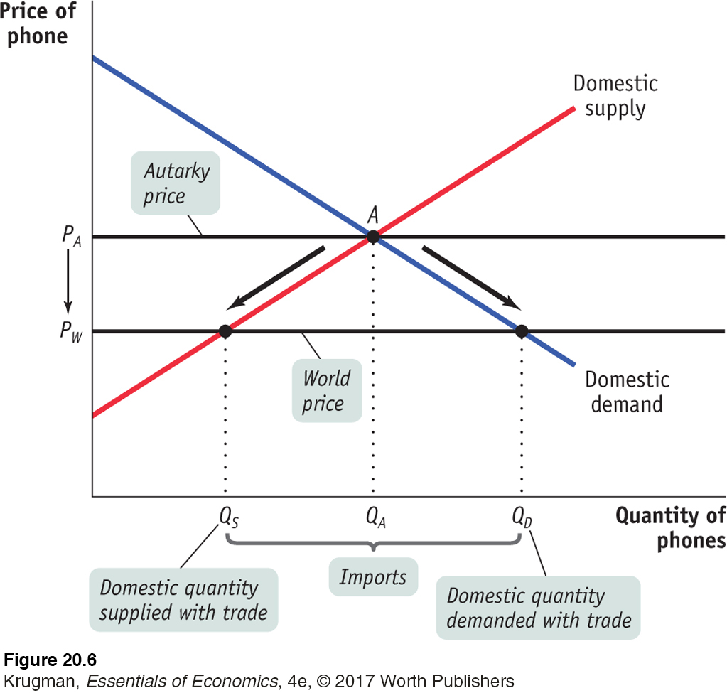
Given that the world price is below the domestic price of a phone, it is profitable for importers to buy phones abroad and resell them domestically. The imported phones increase the supply of phones in the domestic market, driving down the domestic market price. Phones will continue to be imported until the domestic price falls to a level equal to the world price.
The result is shown in Figure 20-6. Because of imports, the domestic price of a phone falls from PA to PW. The quantity of phones demanded by domestic consumers rises from QA to QD, and the quantity supplied by domestic producers falls from QA to QS. The difference between the domestic quantity demanded and the domestic quantity supplied, QD − QS, is filled by imports.
Now let’s turn to the effects of imports on consumer surplus and producer surplus. Because imports of phones lead to a fall in their domestic price, consumer surplus rises and producer surplus falls. Figure 20-7 shows how this works. We label four areas: W, X, Y, and Z. The autarky consumer surplus we identified in Figure 20-5 corresponds to W, and the autarky producer surplus corresponds to the sum of X and Y. The fall in the domestic price to the world price leads to an increase in consumer surplus; it increases by X and Z, so consumer surplus now equals the sum of W, X, and Z. At the same time, producers lose X in surplus, so producer surplus now equals only Y.

The table in Figure 20-7 summarizes the changes in consumer and producer surplus when the phone market is opened to imports. Consumers gain surplus equal to the areas X + Z. Producers lose surplus equal to X. So the sum of producer and consumer surplus—
However, we have also learned that although the country as a whole gains, some groups—
We turn next to the case in which a country exports a good.
The Effects of Exports
Figure 20-8 shows the effects on a country when it exports a good, in this case trucks. For this example, we assume that unlimited quantities of trucks can be sold abroad at a given world price, PW, which is higher than the price that would prevail in the domestic market in autarky, PA.
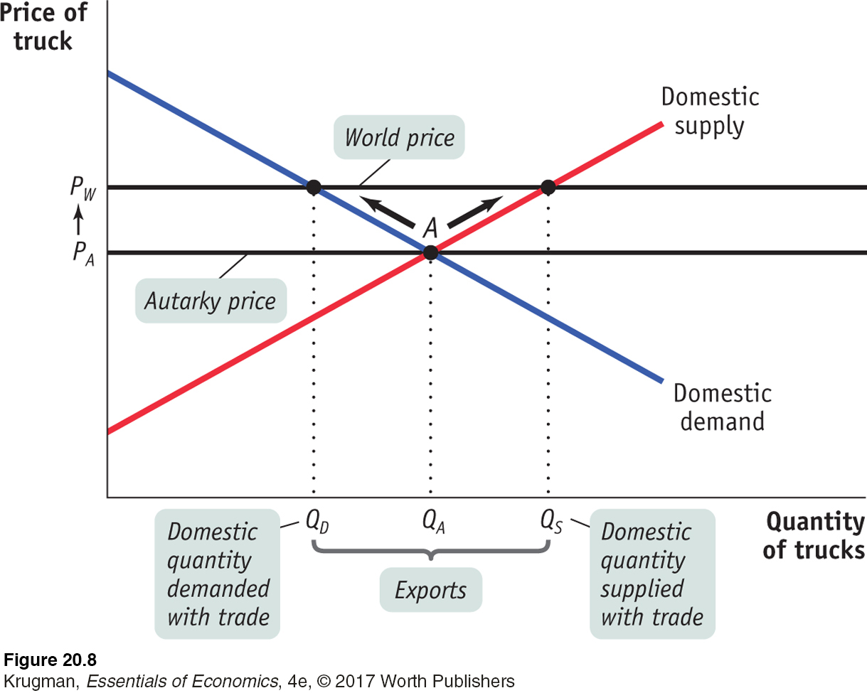
The higher world price makes it profitable for exporters to buy trucks domestically and sell them overseas. The purchases of domestic trucks drive the domestic price up until it is equal to the world price. As a result, the quantity demanded by domestic consumers falls from QA to QD and the quantity supplied by domestic producers rises from QA to QS. This difference between domestic production and domestic consumption, QS − QD, is exported.
Like imports, exports lead to an overall gain in total surplus for the exporting country but also create losers as well as winners. Figure 20-9 shows the effects of truck exports on producer and consumer surplus. In the absence of trade, the price of each truck would be PA. Consumer surplus in the absence of trade is the sum of areas W and X, and producer surplus is area Y. As a result of trade, price rises from PA to PW, consumer surplus falls to W, and producer surplus rises to Y + X + Z. So producers gain X + Z, consumers lose X, and, as shown in the table accompanying the figure, the economy as a whole gains total surplus in the amount of Z.
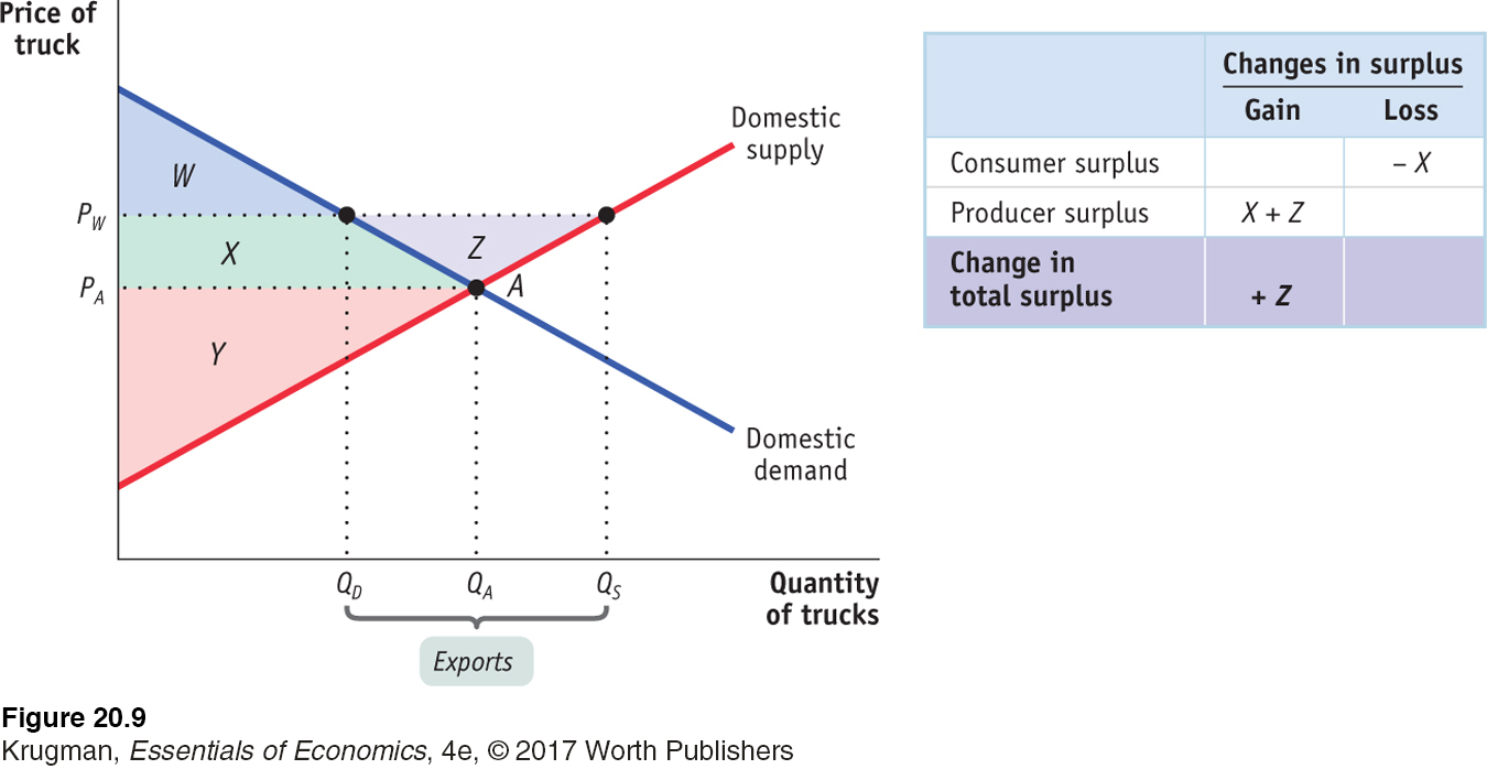
We have learned, then, that imports of a particular good hurt domestic producers of that good but help domestic consumers, whereas exports of a particular good hurt domestic consumers of that good but help domestic producers. In each case, the gains are larger than the losses.
International Trade and Wages
So far we have focused on the effects of international trade on producers and consumers in a particular industry. For many purposes this is a very helpful approach. However, producers and consumers are not the only parts of society affected by trade—
Moreover, the effects of trade aren’t limited to just those industries that export or compete with imports because factors of production can often move between industries. So now we turn our attention to the long-
To begin our analysis, consider the position of Maria, an accountant at West Coast Phone Production, Inc. If the economy is opened up to imports of phones from China, the domestic phone industry will contract, and it will hire fewer accountants. But accounting is a profession with employment opportunities in many industries, and Maria might well find a better job in the automobile industry, which expands as a result of international trade. So it may not be appropriate to think of her as a producer of phones who is hurt by competition from imported parts. Rather, we should think of her as an accountant who is affected by phone imports only to the extent that these imports change the wages of accountants in the economy as a whole.
The wage rate of accountants is a factor price—
Earlier we described the Heckscher–Ohlin model of trade, which states that comparative advantage is determined by a country’s factor endowment. This model also suggests how international trade affects factor prices in a country: compared to autarky, international trade tends to raise the prices of factors that are abundantly available and reduce the prices of factors that are scarce.
We won’t work this out in detail, but the idea is simple. The prices of factors of production, like the prices of goods and services, are determined by supply and demand. If international trade increases the demand for a factor of production, that factor’s price will rise; if international trade reduces the demand for a factor of production, that factor’s price will fall.
Exporting industries produce goods and services that are sold abroad.
Import-
Now think of a country’s industries as consisting of two kinds: exporting industries, which produce goods and services that are sold abroad, and import-
In addition, the Heckscher–Ohlin model says that a country tends to export goods that are intensive in its abundant factors and to import goods that are intensive in its scarce factors. So international trade tends to increase the demand for factors that are abundant in our country compared with other countries, and to decrease the demand for factors that are scarce in our country compared with other countries. As a result, the prices of abundant factors tend to rise, and the prices of scarce factors tend to fall as international trade grows.
In other words, international trade tends to redistribute income toward a country’s abundant factors and away from its less abundant factors.
U.S. exports tend to be human-
This effect has been a source of much concern in recent years. Wage inequality—the gap between the wages of high-
How important are these effects? In some historical episodes, the impacts of international trade on factor prices have been very large. As we explain in the following Economics in Action, the opening of transatlantic trade in the late nineteenth century had a large negative impact on land rents in Europe, hurting landowners but helping workers and owners of capital.
The effects of trade on wages in the United States have generated considerable controversy in recent years. Most economists who have studied the issue agree that growing imports of labor-
ECONOMICS in Action
Trade, Wages, and Land Prices in the Nineteenth Century
![]() | interactive activity
| interactive activity
Beginning around 1870, there was an explosive growth of world trade in agricultural products, based largely on the steam engine. Steam-
This opening up of international trade led to higher prices of agricultural products, such as wheat, in exporting countries and a decline in their prices in importing countries. Notably, the difference between wheat prices in the midwestern United States and England plunged.
The change in agricultural prices created winners and losers on both sides of the Atlantic as factor prices adjusted. In England, land prices fell by half compared with average wages; landowners found their purchasing power sharply reduced, but workers benefited from cheaper food. In the United States, the reverse happened: land prices doubled compared with wages. Landowners did very well, but workers found the purchasing power of their wages dented by rising food prices.
Quick Review
The intersection of the domestic demand curve and the domestic supply curve determines the domestic price of a good. When a market is opened to international trade, the domestic price is driven to equal the world price.
If the world price is lower than the autarky price, trade leads to imports and the domestic price falls to the world price. There are overall gains from international trade because the gain in consumer surplus exceeds the loss in producer surplus.
If the world price is higher than the autarky price, trade leads to exports and the domestic price rises to the world price. There are overall gains from international trade because the gain in producer surplus exceeds the loss in consumer surplus.
Trade leads to an expansion of exporting industries, which increases demand for a country’s abundant factors, and a contraction of import-
competing industries, which decreases demand for its scarce factors.
Check Your Understanding 20-2
Question 20.3
1. Due to a strike by truckers, trade in food between the United States and Mexico is halted. In autarky, the price of Mexican grapes is lower than that of U.S. grapes. Using a diagram of the U.S. domestic demand curve and the U.S. domestic supply curve for grapes, explain the effect of the strike on the following.
U.S. grape consumers’ surplus
U.S. grape producers’ surplus
U.S. total surplus
In the accompanying diagram, PA is the U.S. price of grapes in autarky and PW is the world price of grapes under international trade. With trade, U.S. consumers pay a price of PW for grapes and consume quantity QD, U.S. grape producers produce quantity QS, and the difference, QD − QS, represents imports of Mexican grapes. As a consequence of the strike by truckers, imports are halted, the price paid by American consumers rises to the autarky price, PA, and U.S. consumption falls to the autarky quantity, QA.
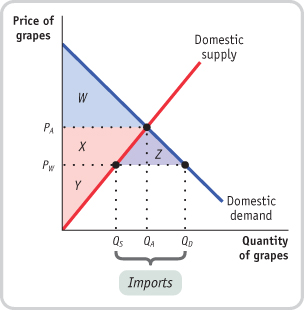
Before the strike, U.S. consumers enjoyed consumer surplus equal to areas W + X + Z. After the strike, their consumer surplus shrinks to W. So consumers are worse off, losing consumer surplus represented by X + Z.
Before the strike, U.S. producers had producer surplus equal to the area Y. After the strike, their producer surplus increases to Y + X. So U.S. producers are better off, gaining producer surplus represented by X.
U.S. total surplus falls as a result of the strike by an amount represented by area Z, the loss in consumer surplus that does not accrue to producers.
Question 20.4
2. What effect do you think the strike will have on Mexican grape producers? Mexican grape pickers? Mexican grape consumers? U.S. grape pickers?
Mexican grape producers are worse off because they lose sales of exported grapes to the United States, and Mexican grape pickers are worse off because they lose the wages that were associated with the lost sales. The lower demand for Mexican grapes caused by the strike implies that the price Mexican consumers pay for grapes falls, making them better off. U.S. grape pickers are better off because their wages increase as a result of the increase of QA − QS in U.S. sales.
Solutions appear at back of book.