5.6 The Benefits and Costs of Taxation
157
An excise tax is a tax on sales of a good or service.
When a government is considering whether to impose a tax or how to design a tax system, it has to weigh the benefits of a tax against its costs. We don’t usually think of a tax as something that provides benefits, but governments need money to provide things people want, such as national defense and health care for those unable to afford it. The benefit of a tax is the revenue it raises for the government to pay for these services. Unfortunately, this benefit comes at a cost—
The Revenue from an Excise Tax
Suppose that the supply and demand for hotel rooms in the city of Potterville are as shown in Figure 5-7. For simplicity, assume that all hotel rooms offer the same features. In the absence of taxes, the equilibrium price of a room is $80.00 per night and the equilibrium quantity of hotel rooms rented is 10,000 per night.
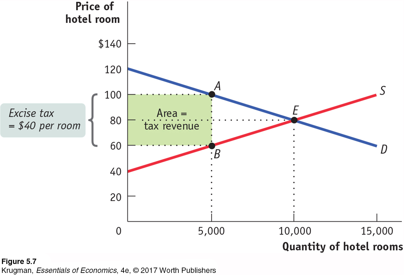
Now suppose that Potterville’s city council imposes an excise tax of $40 per night on hotel rooms—
How much revenue will the government collect from this excise tax? In this case, the revenue is equal to the area of the shaded rectangle in Figure 5-7.
To see why this area represents the revenue collected by a $40 tax on hotel rooms, notice that the height of the rectangle is $40, equal to the tax per room. It is also, as we’ve seen, the size of the wedge that the tax drives between the supply price (the price received by producers) and the demand price (the price paid by consumers). Meanwhile, the width of the rectangle is 5,000 rooms, equal to the equilibrium quantity of rooms given the $40 tax. With that information, we can make the following calculations.
The tax revenue collected is:
Tax revenue = $40 per room × 5,000 rooms = $200,000
158
The area of the shaded rectangle is:
Area = Height × Width = $40 per room × 5,000 rooms = $200,000
or
Tax revenue = Area of shaded rectangle
This is a general principle: The revenue collected by an excise tax is equal to the area of the rectangle whose height is the tax wedge between the supply and demand curves and whose width is the quantity transacted under the tax.
Tax Rates and Revenue
A tax rate is the amount of tax people are required to pay per unit of whatever is being taxed.
In Figure 5-7, $40 per room is the tax rate on hotel rooms. A tax rate is the amount of tax levied per unit of whatever is being taxed. Sometimes tax rates are defined in terms of dollar amounts per unit of a good or service; for example, $2.46 per pack of cigarettes sold. In other cases, they are defined as a percentage of the price; for example, the payroll tax is 15.3% of a worker’s earnings up to $117,000.
There’s obviously a relationship between tax rates and revenue. That relationship is not, however, one-
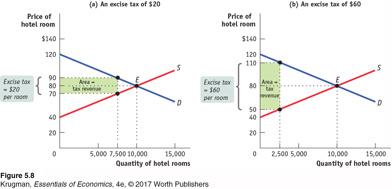
We can illustrate these points using our hotel room example. Figure 5-7 showed the revenue the government collects from a $40 tax on hotel rooms. Figure 5-8 shows the revenue the government would collect from two alternative tax rates—
Panel (a) of Figure 5-8 shows the case of a $20 tax, equal to half the tax rate illustrated in Figure 5-7. At this lower tax rate, 7,500 rooms are rented, generating tax revenue of:
Tax revenue = $20 per room × 7,500 rooms = $150,000
Recall that the tax revenue collected from a $40 tax rate is $200,000. So the revenue collected from a $20 tax rate, $150,000, is only 75% of the amount collected when the tax rate is twice as high ($150,000/$200,000 × 100 = 75%). To put it another way, a 100% increase in the tax rate from $20 to $40 per room leads to only a one-
Panel (b) depicts what happens if the tax rate is raised from $40 to $60 per room, leading to a fall in the number of rooms rented from 5,000 to 2,500. The revenue collected at a $60 per room tax rate is:
Tax revenue = $60 per room × 2,500 rooms = $150,000
This is also less than the revenue collected by a $40 per room tax. So raising the tax rate from $40 to $60 actually reduces revenue. More precisely, in this case raising the tax rate by 50% (($60 − $40)/$40 × 100 = 50%) lowers the tax revenue by 25% (($150,000 − $200,000)/$200,000 × 100 = −25%). Why did this happen? Because the fall in tax revenue caused by the reduction in the number of rooms rented more than offset the increase in the tax revenue caused by the rise in the tax rate. In other words, setting a tax rate so high that it deters a significant number of transactions will likely lead to a fall in tax revenue.
159
One way to think about the revenue effect of increasing an excise tax is that the tax increase affects tax revenue in two ways. On one side, the tax increase means that the government raises more revenue for each unit of the good sold, which other things equal would lead to a rise in tax revenue. On the other side, the tax increase reduces the quantity of sales, which other things equal would lead to a fall in tax revenue. The end result depends both on the price elasticities of supply and demand and on the initial level of the tax.
If the price elasticities of both supply and demand are low, the tax increase won’t reduce the quantity of the good sold very much, so tax revenue will definitely rise. If the price elasticities are high, the result is less certain; if they are high enough, the tax reduces the quantity sold so much that tax revenue falls. Also, if the initial tax rate is low, the government doesn’t lose much revenue from the decline in the quantity of the good sold, so the tax increase will definitely increase tax revenue. If the initial tax rate is high, the result is again less certain. Tax revenue is likely to fall or rise very little from a tax increase only in cases where the price elasticities are high and there is already a high tax rate.
The possibility that a higher tax rate can reduce tax revenue, and the corresponding possibility that cutting taxes can increase tax revenue, is a basic principle of taxation that policy makers take into account when setting tax rates. That is, when considering a tax created for the purpose of raising revenue (in contrast to taxes created to discourage undesirable behavior, known as “sin taxes”), a well-
In the real world, however, policy makers aren’t always well informed, but they usually aren’t complete fools either. That’s why it’s very hard to find real-
160
The Costs of Taxation
What is the cost of a tax? You might be inclined to answer that it is the money taxpayers pay to the government. In other words, you might believe that the cost of a tax is the tax revenue collected. But suppose the government uses the tax revenue to provide services that taxpayers want. Or suppose that the government simply hands the tax revenue back to taxpayers. Would we say in those cases that the tax didn’t actually cost anything?
No—
For example, we know from the supply and demand curves that there are some potential guests who would be willing to pay up to $90 per night and some hotel owners who would be willing to supply rooms if they received at least $70 per night. If these two sets of people were allowed to trade with each other without the tax, they would engage in mutually beneficial transactions—
But such deals would be illegal, because the $40 tax would not be paid. In our example, 5,000 potential hotel room rentals that would have occurred in the absence of the tax, to the mutual benefit of guests and hotel owners, do not take place because of the tax.
So an excise tax imposes costs over and above the tax revenue collected in the form of inefficiency, which occurs because the tax discourages mutually beneficial transactions. As we learned in Chapter 4, the cost to society of this kind of inefficiency—
161
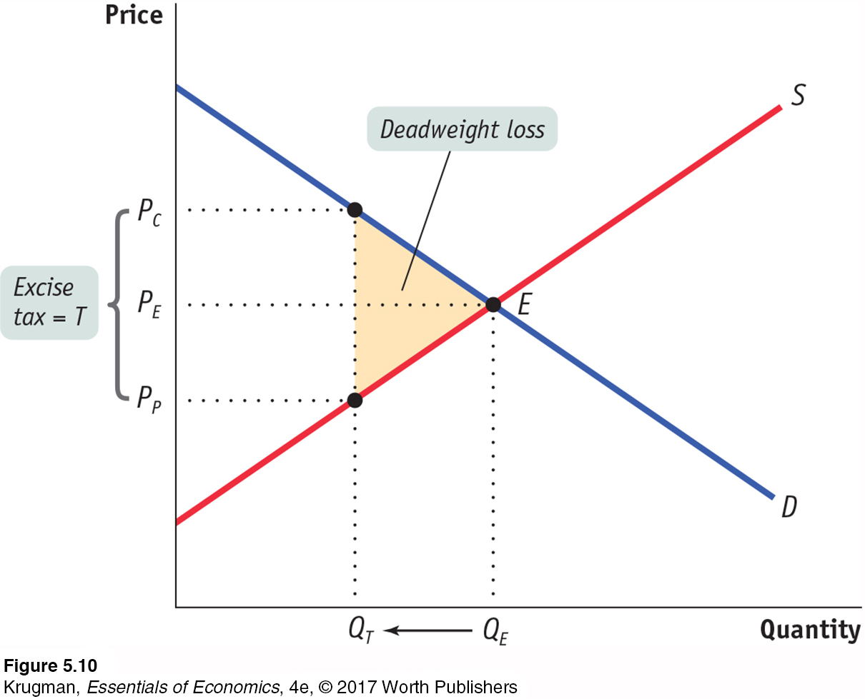
To measure the deadweight loss from a tax, we turn to the concepts of producer and consumer surplus. Figure 5-9 shows the effects of an excise tax on consumer and producer surplus. In the absence of the tax, the equilibrium is at E and the equilibrium price and quantity are PE and QE, respectively. An excise tax drives a wedge equal to the amount of the tax between the price received by producers and the price paid by consumers, reducing the quantity sold. In this case, where the tax is T dollars per unit, the quantity sold falls to QT. The price paid by consumers rises to PC, the demand price of the reduced quantity, QT, and the price received by producers falls to PP, the supply price of that quantity. The difference between these prices, PC − PP, is equal to the excise tax, T.
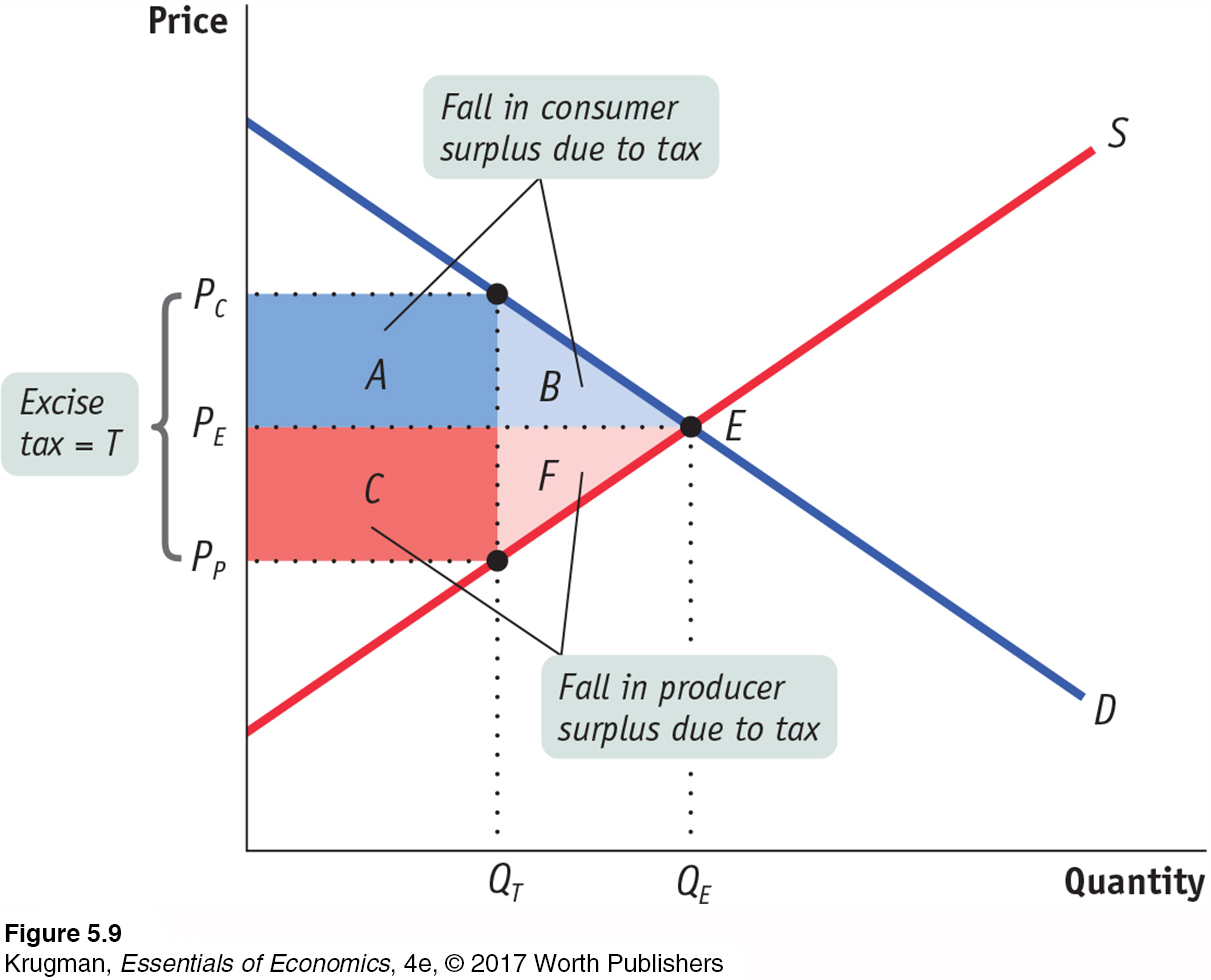
The rise in the price paid by consumers causes a loss equal to the sum of the areas of a rectangle and a triangle: the dark blue rectangle labeled A and the area of the light blue triangle labeled B in Figure 5-9.
Meanwhile, the fall in the price received by producers leads to a fall in producer surplus. This, too, is equal to the sum of the areas of a rectangle and a triangle. The loss in producer surplus is the sum of the areas of the red rectangle labeled C and the pink triangle labeled F in Figure 5-9.
Of course, although consumers and producers are hurt by the tax, the government gains revenue. The revenue the government collects is equal to the tax per unit sold, T, multiplied by the quantity sold, QT. This revenue is equal to the area of a rectangle QT wide and T high. And we already have that rectangle in the figure: it is the sum of rectangles A and C. So the government gains part of what consumers and producers lose from an excise tax.
But a portion of the loss to producers and consumers from the tax is not offset by a gain to the government—
Figure 5-10 is a version of Figure 5-9 that leaves out rectangles A (the surplus shifted from consumers to the government) and C (the surplus shifted from producers to the government) and shows only the deadweight loss, here drawn as a triangle shaded yellow. The base of that triangle is equal to the tax wedge, T; the height of the triangle is equal to the reduction in the quantity transacted due to the tax, QE − QT. Clearly, the larger the tax wedge and the larger the reduction in the quantity transacted, the greater the inefficiency from the tax.
162
But also note an important, contrasting point: if the excise tax somehow didn’t reduce the quantity bought and sold in this market—
Using a triangle to measure deadweight loss is a technique used in many economic applications. For example, triangles are used to measure the deadweight loss produced by types of taxes other than excise taxes. They are also used to measure the deadweight loss produced by monopoly, another kind of market distortion. And deadweight-
The administrative costs of a tax are the resources used for its collection, for the method of payment, and for any attempts to evade the tax.
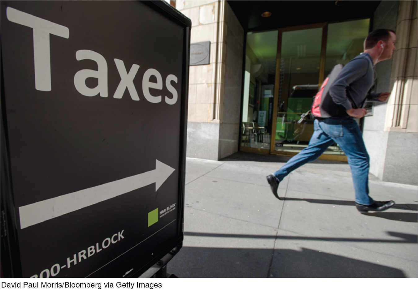
In considering the total amount of inefficiency caused by a tax, we must also take into account something not shown in Figure 5-10: the resources actually used by the government to collect the tax, and by taxpayers to pay it, over and above the amount of the tax. These lost resources are called the administrative costs of the tax. The most familiar administrative cost of the U.S. tax system is the time individuals spend filling out their income tax forms or the money they pay for tax return preparation services like those provided by H&R Block and companies like it. (The latter is considered an inefficiency from the point of view of society because resources spent on return preparation could be used for other, non-
Included in the administrative costs that taxpayers incur are resources used to evade the tax, both legally and illegally. The costs of operating the Internal Revenue Service, the arm of the federal government tasked with collecting the federal income tax, are actually quite small in comparison to the administrative costs paid by taxpayers.
So the total inefficiency caused by a tax is the sum of its deadweight loss and its administrative costs. The general rule for economic policy is that, other things equal, a tax system should be designed to minimize the total inefficiency it imposes on society. In practice, other considerations also apply, but this principle nonetheless gives valuable guidance. Administrative costs are usually well known, more or less determined by the current technology of collecting taxes (for example, filing paper returns versus filing electronically). But how can we predict the size of the deadweight loss associated with a given tax? Not surprisingly, as in our analysis of the incidence of a tax, the price elasticities of supply and demand play crucial roles in making such a prediction.
Elasticities and the Deadweight Loss of a Tax
We know that the deadweight loss from an excise tax arises because it prevents some mutually beneficial transactions from occurring. In particular, the producer and consumer surplus that is forgone because of these missing transactions is equal to the size of the deadweight loss itself. This means that the larger the number of transactions that are prevented by the tax, the larger the deadweight loss.
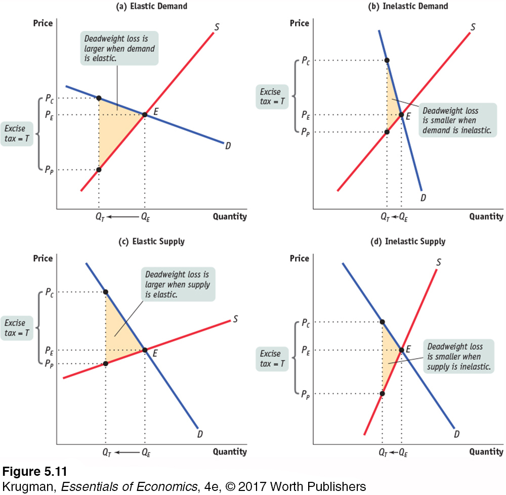
This fact gives us an important clue in understanding the relationship between elasticity and the size of the deadweight loss from a tax. Recall that when demand or supply is elastic, the quantity demanded or the quantity supplied is relatively responsive to changes in the price. So a tax imposed on a good for which either demand or supply, or both, is elastic will cause a relatively large decrease in the quantity transacted and a relatively large deadweight loss. And when we say that demand or supply is inelastic, we mean that the quantity demanded or the quantity supplied is relatively unresponsive to changes in the price.
163
As a result, a tax imposed when demand or supply, or both, is inelastic will cause a relatively small decrease in the quantity transacted and a relatively small deadweight loss.
The four panels of Figure 5-11 illustrate the positive relationship between a good’s price elasticity of either demand or supply and the deadweight loss from taxing that good. Each panel represents the same amount of tax imposed but on a different good; the size of the deadweight loss is given by the area of the shaded triangle. In panel (a), the deadweight-
164
The implication of this result is clear: if you want to minimize the efficiency costs of taxation, you should choose to tax only those goods for which demand or supply, or both, is relatively inelastic. For such goods, a tax has little effect on behavior because behavior is relatively unresponsive to changes in the price. In the extreme case in which demand is perfectly inelastic (a vertical demand curve), the quantity demanded is unchanged by the imposition of the tax. As a result, the tax imposes no deadweight loss. Similarly, if supply is perfectly inelastic (a vertical supply curve), the quantity supplied is unchanged by the tax and there is also no deadweight loss.
So if the goal in choosing whom to tax is to minimize deadweight loss, then taxes should be imposed on goods and services that have the most inelastic response—
ECONOMICS in Action
Taxing the Marlboro Man
![]() | interactive activity
| interactive activity
One of the most important excise taxes in the United States is the tax on cigarettes. The federal government imposes a tax of $1.01 a pack; state governments impose taxes that range from $0.17 cents a pack in Missouri to $4.35 a pack in New York; and many cities impose further taxes. In general, tax rates on cigarettes have increased over time, because more and more governments have seen them not just as a source of revenue but as a way to discourage smoking. But the rise in cigarette taxes has not been gradual. Usually, once a state government decides to raise cigarette taxes, it raises them a lot—
| State | Year | Increase in tax (per pack) |
New state tax (per pack) |
Change in quantity transacted |
Change in tax revenue |
| Mississippi | 2009 | $0.50 | $0.68 | −22.8% | 188.3% |
| Hawaii | 2009 | 0.60 | 2.60 | −1.3 | −14.5 |
| New Mexico | 2010 | 0.75 | 1.66 | −7.8 | 67.5 |
| Florida | 2010 | 1.00 | 2.00 | −27.8 | 193.2 |
| Washington | 2010 | 1.00 | 3.03 | −20.5 | 17.0 |
Data from: Orzechowski & Walker, Tax Burden on Tobacco. U.S. Alcohol and Tobacco Tax and Trade Bureau.
Table 5-4 shows the results of big increases in cigarette taxes. In each case, sales fell, just as our analysis predicts. Although it’s theoretically possible for tax revenue to fall after such a large tax increase, in reality tax revenue rose in each case. That’s because cigarettes have a low price elasticity of demand.
165
Quick Review
An excise tax generates tax revenue equal to the tax rate times the number of units of the good or service transacted but reduces consumer and producer surplus.
The government tax revenue collected is less than the loss in total surplus because the tax creates inefficiency by discouraging some mutually beneficial transactions.
The difference between the tax revenue from an excise tax and the reduction in total surplus is the deadweight loss from the tax. The total amount of inefficiency resulting from a tax is equal to the deadweight loss plus the administrative costs of the tax.
The larger the number of transactions prevented by a tax, the larger the deadweight loss. As a result, taxes on goods with a greater price elasticity of supply or demand, or both, generate higher deadweight losses. There is no deadweight loss when the number of transactions is unchanged by the tax.
Check Your Understanding 5-
Question 5.13
1. The accompanying table shows five consumers’ willingness to pay for one can of diet soda each as well as five producers’ costs of selling one can of diet soda each. Each consumer buys at most one can of soda; each producer sells at most one can of soda. The government asks your advice about the effects of an excise tax of $0.40 per can of diet soda. Assume that there are no administrative costs from the tax.
| Consumer | Willingness to pay |
Producer | Cost |
| Ana | $0.70 | Zhang | $0.10 |
| Bernice | 0.60 | Yves | 0.20 |
| Chizuko | 0.50 | Xavier | 0.30 |
| Dagmar | 0.40 | Walter | 0.40 |
| Ella | 0.30 | Vern | 0.50 |
Without the excise tax, what is the equilibrium price and the equilibrium quantity of soda transacted?
Without the excise tax, Zhang, Yves, Xavier, and Walter sell, and Ana, Bernice, Chizuko, and Dagmar buy one can of soda each, at $0.40 per can. So the quantity bought and sold is 4.
The excise tax raises the price paid by consumers post-
tax to $0.60 and lowers the price received by producers post- tax to $0.20. With the excise tax, what is the quantity of soda transacted? At a price to consumers of $0.60, only Ana and Bernice are willing to buy a can of soda. At a price paid to producers of only $0.20, only Zhang and Yves are willing to sell. So the quantity bought and sold is 2.
Without the excise tax, how much individual consumer surplus does each of the consumers gain? How much with the tax? How much total consumer surplus is lost as a result of the tax?
Without the excise tax, Ana’s individual consumer surplus is $0.70 − $0.40 = $0.30, Bernice’s is $0.60 − $0.40 = $0.20, Chizuko’s is $0.50 − $0.40 = $0.10, and Dagmar’s is $0.40 − $0.40 = $0.00. Total consumer surplus is $0.30 + $0.20 + $0.10 + $0.00 = $0.60. With the tax, Ana’s individual consumer surplus is $0.70 −$0.60 = $0.10 and Bernice’s is $0.60 − $0.60 = $0.00. Total consumer surplus post-
tax is $0.10 + $0.00 = $0.10. So the total consumer surplus lost because of the tax is $0.60 − $0.10 = $0.50. Without the excise tax, how much individual producer surplus does each of the producers gain? How much with the tax? How much total producer surplus is lost as a result of the tax?
Without the excise tax, Zhang’s individual producer surplus is $0.40 − $0.10 = $0.30, Yves’s is $0.40 − $0.20 = $0.20, Xavier’s is $0.40 − $0.30 = $0.10, and Walter’s is $0.40 − $0.40 = $0.00. Total producer surplus is $0.30 + $0.20 + $0.10 + $0.00 = $0.60. With the tax, Zhang’s individual producer surplus is $0.20 − $0.10 = $0.10 and Yves’s is $0.20 − $0.20 = $0.00. Total producer surplus post-
tax is $0.10 + $0.00 = $0.10. So the total producer surplus lost because of the tax is $0.60 − $0.10 = $0.50. How much government revenue does the excise tax create?
With the tax, two cans of soda are sold, so the government tax revenue from this excise tax is 2 × $0.40 = $0.80.
What is the deadweight loss from the imposition of this excise tax?
Total surplus without the tax is $0.60 + $0.60 = $1.20. With the tax, total surplus is $0.10 + $0.10 = $0.20, and government tax revenue is $0.80. So deadweight loss from this excise tax is $1.20 − ($0.20 + $0.80) = $0.20.
Question 5.14
2. In each of the following cases, focus on the price elasticity of demand and use a diagram to illustrate the likely size—
Gasoline
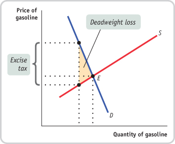
The demand for gasoline is inelastic because there is no close substitute for gasoline itself and it is difficult for drivers to arrange substitutes for driving, such as taking public transportation. As a result, the deadweight loss from a tax on gasoline would be relatively small, as shown in the accompanying diagram.
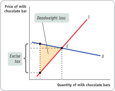
Milk chocolate bars
The demand for milk chocolate bars is elastic because there are close substitutes: dark chocolate bars, milk chocolate kisses, and so on. As a result, the deadweight loss from a tax on milk chocolate bars would be relatively large, as shown in the accompanying diagram.
Solutions appear at back of book.