Short-Run versus Long-Run Costs
Up to this point, we have treated fixed cost as completely outside the control of a firm because we have focused on the short run. But as we noted earlier, all inputs are variable in the long run: this means that in the long run fixed cost may also be varied. In the long run, in other words, a firm’s fixed cost becomes a variable it can choose. For example, given time, Selena’s Gourmet Salsas can acquire additional food-preparation equipment or dispose of some of its existing equipment. In this section, we will examine how a firm’s costs behave in the short run and in the long run. We will also see that the firm will choose its fixed cost in the long run based on the level of output it expects to produce.
Let’s begin by supposing that Selena’s Gourmet Salsas is considering whether to acquire additional food-preparation equipment. Acquiring additional machinery will affect its total cost in two ways. First, the firm will have to either rent or buy the additional equipment; either way, that will mean higher fixed cost in the short run. Second, if the workers have more equipment, they will be more productive: fewer workers will be needed to produce any given output, so variable cost for any given output level will be reduced.
The table in Figure 6-11 shows how acquiring an additional machine affects costs. In our original example, we assumed that Selena’s Gourmet Salsas had a fixed cost of $108. The left half of the table shows variable cost as well as total cost and average total cost assuming a fixed cost of $108. The average total cost curve for this level of fixed cost is given by ATC1 in Figure 6-11. Let’s compare that to a situation in which the firm buys additional food-preparation equipment, doubling its fixed cost to $216 but reducing its variable cost at any given level of output. The right half of the table shows the firm’s variable cost, total cost, and average total cost with this higher level of fixed cost. The average total cost curve corresponding to $216 in fixed cost is given by ATC2 in Figure 6-11.
FIGURE 6-11 Choosing the Level of Fixed Cost for Selena’s Gourmet Salsas

From the figure you can see that when output is small, 4 cases of salsa per day or fewer, average total cost is smaller when Selena forgoes the additional equipment and maintains the lower fixed cost of $108: ATC1 lies below ATC2. For example, at 3 cases per day, average total cost is $72 without the additional machinery and $90 with the additional machinery. But as output increases beyond 4 cases per day, the firm’s average total cost is lower if it acquires the additional equipment, raising its fixed cost to $216. For example, at 9 cases of salsa per day, average total cost is $120 when fixed cost is $108 but only $78 when fixed cost is $216.
Why does average total cost change like this when fixed cost increases? When output is low, the increase in fixed cost from the additional equipment outweighs the reduction in variable cost from higher worker productivity—that is, there are too few units of output over which to spread the additional fixed cost. So if Selena plans to produce 4 or fewer cases per day, she would be better off choosing the lower level of fixed cost, $108, to achieve a lower average total cost of production. When planned output is high, however, she should acquire the additional machinery.
In general, for each output level there is some choice of fixed cost that minimizes the firm’s average total cost for that output level. So when the firm has a desired output level that it expects to maintain over time, it should choose the level of fixed cost optimal for that level—that is, the level of fixed cost that minimizes its average total cost.
Now that we are studying a situation in which fixed cost can change, we need to take time into account when discussing average total cost. All of the average total cost curves we have considered until now are defined for a given level of fixed cost—that is, they are defined for the short run, the period of time over which fixed cost doesn’t vary. To reinforce that distinction, for the rest of this chapter we will refer to these average total cost curves as “short-run average total cost curves.”
For most firms, it is realistic to assume that there are many possible choices of fixed cost, not just two. The implication: for such a firm, many possible short-run average total cost curves will exist, each corresponding to a different choice of fixed cost and so giving rise to what is called a firm’s “family” of short-run average total cost curves.
At any given point in time, a firm will find itself on one of its short-run cost curves, the one corresponding to its current level of fixed cost; a change in output will cause it to move along that curve. If the firm expects that change in output level to be long-standing, then it is likely that the firm’s current level of fixed cost is no longer optimal. Given sufficient time, it will want to adjust its fixed cost to a new level that minimizes average total cost for its new output level. For example, if Selena had been producing 2 cases of salsa per day with a fixed cost of $108 but found herself increasing her output to 8 cases per day for the foreseeable future, then in the long run she should purchase more equipment and increase her fixed cost to a level that minimizes average total cost at the 8-cases-per-day output level.
The long-run average total cost curve shows the relationship between output and average total cost when fixed cost has been chosen to minimize average total cost for each level of output.
Suppose we do a thought experiment and calculate the lowest possible average total cost that can be achieved for each output level if the firm were to choose its fixed cost for each output level. Economists have given this thought experiment a name: the long-run average total cost curve. Specifically, the long-run average total cost curve, or LRATC, is the relationship between output and average total cost when fixed cost has been chosen to minimize average total cost for each level of output. If there are many possible choices of fixed cost, the long-run average total cost curve will have the familiar, smooth U shape, as shown by LRATC in Figure 6-12.
FIGURE 6-12 Short-Run and Long-Run Average Total Cost Curves

We can now draw the distinction between the short run and the long run more fully. In the long run, when a producer has had time to choose the fixed cost appropriate for its desired level of output, that producer will be at some point on the long-run average total cost curve. But if the output level is altered, the firm will no longer be on its long-run average total cost curve and will instead be moving along its current short-run average total cost curve. It will not be on its long-run average total cost curve again until it readjusts its fixed cost for its new output level.
Figure 6-12 illustrates this point. The curve ATC3 shows short-run average total cost if Selena has chosen the level of fixed cost that minimizes average total cost at an output of 3 cases of salsa per day. This is confirmed by the fact that at 3 cases per day, ATC3 touches LRATC, the long-run average total cost curve. Similarly, ATC6 shows short-run average total cost if Selena has chosen the level of fixed cost that minimizes average total cost if her output is 6 cases per day. It touches LRATC at 6 cases per day. And ATC9 shows short-run average total cost if Selena has chosen the level of fixed cost that minimizes average total cost if her output is 9 cases per day. It touches LRATC at 9 cases per day.
Suppose that Selena initially chose to be on ATC6. If she actually produces 6 cases of salsa per day, her firm will be at point C on both its short-run and long-run average total cost curves. Suppose, however, that Selena ends up producing only 3 cases of salsa per day. In the short run, her average total cost is indicated by point B on ATC6; it is no longer on LRATC. If Selena had known that she would be producing only 3 cases per day, she would have been better off choosing a lower level of fixed cost, the one corresponding to ATC3, thereby achieving a lower average total cost. Then her firm would have found itself at point A on the long-run average total cost curve, which lies below point B.
Suppose, conversely, that Selena ends up producing 9 cases per day even though she initially chose to be on ATC6. In the short run her average total cost is indicated by point Y on ATC6. But she would be better off purchasing more equipment and incurring a higher fixed cost in order to reduce her variable cost and move to ATC9. This would allow her to reach point X on the long-run average total cost curve, which lies below Y.
The distinction between short-run and long-run average total costs is extremely important in making sense of how real firms operate over time. A company that has to increase output suddenly to meet a surge in demand will typically find that in the short run its average total cost rises sharply because it is hard to get extra production out of existing facilities. But given time to build new factories or add machinery, short-run average total cost falls.
Returns to Scale
There are increasing returns to scale when long-run average total cost declines as output increases.
What determines the shape of the long-run average total cost curve? The answer is that scale, the size of a firm’s operations, is often an important determinant of its long-run average total cost of production. Firms that experience scale effects in production find that their long-run average total cost changes substantially depending on the quantity of output they produce. There are increasing returns to scale (also known as economies of scale) when long-run average total cost declines as output increases. As you can see in Figure 6-12, Selena’s Gourmet Salsas experiences increasing returns to scale over output levels ranging from 0 up to 5 cases of salsa per day—the output levels over which the long-run average total cost curve is declining. In contrast, there are decreasing returns to scale (also known as diseconomies of scale) when long-run average total cost increases as output increases. For Selena’s Gourmet Salsas, decreasing returns to scale occur at output levels greater than 7 cases, the output levels over which its long-run average total cost curve is rising. There is also a third possible relationship between long-run average total cost and scale: firms experience constant returns to scale when long-run average total cost is constant as output increases. In this case, the firm’s long-run average total cost curve is horizontal over the output levels for which there are constant returns to scale. As you can see in Figure 6-12, Selena’s Gourmet Salsas has constant returns to scale when it produces anywhere from 5 to 7 cases of salsa per day.
There are decreasing returns to scale when long-run average total cost increases as output increases.
There are constant returns to scale when long-run average total cost is constant as output increases.
A good is subject to a network externality when the value of the good to an individual is greater when a large number of other people also use that good.
What explains these scale effects in production? The answer ultimately lies in the firm’s technology of production. Increasing returns often arise from the increased specialization that larger output levels allow—a larger scale of operation means that individual workers can limit themselves to more specialized tasks, becoming more skilled and efficient at doing them. Another source of increasing returns is very large initial setup cost; in some industries—such as auto manufacturing, electricity generating, or petroleum refining—incurring a high fixed cost in the form of plant and equipment is necessary to produce any output. A third source of increasing returns, found in certain high-tech industries such as software development, is known as a network externality. The classic example is computer operating systems. Worldwide, most personal computers run on Microsoft Windows. Although many believe that Apple has a superior operating system, the wider use of Windows in the early days of personal computers attracted more software development and technical support, giving it lasting dominance. As we’ll see in Chapter 8, where we study monopoly, increasing returns have very important implications for how firms and industries interact and behave.
Decreasing returns—the opposite scenario—typically arise in large firms due to problems of coordination and communication: as the firm grows in size, it becomes ever more difficult and so more costly to communicate and to organize its activities. Although increasing returns induce firms to get larger, decreasing returns tend to limit their size. And when there are constant returns to scale, scale has no effect on a firm’s long-run average total cost: it is the same regardless of whether the firm produces 1 unit or 100,000 units.
Summing Up Costs: The Short and Long of It
If a firm is to make the best decisions about how much to produce, it has to understand how its costs relate to the quantity of output it chooses to produce. Table 6-3 provides a quick summary of the concepts and measures of cost you have learned about.
TABLE 6-3 Concepts and Measures of Cost

There’S No Business Like Snow Business

Anyone who has lived both in a snowy city, like Chicago, and in a city that only occasionally experiences significant snowfall, like Washington, D.C., is aware of the differences in total cost that arise from making different choices about fixed cost.
In Washington, even a minor snowfall—say, an inch or two overnight—is enough to create chaos during the next morning’s commute. The same snowfall in Chicago has hardly any effect at all. The reason is not that Washingtonians are wimps and Chicagoans are made of sterner stuff; it is that Washington, where it rarely snows, has only a fraction as many snowplows and other snowclearing equipment as cities where heavy snow is a fact of life.
In this sense Washington and Chicago are like two producers who expect to produce different levels of output, where the “output” is snow removal. Washington, which rarely has significant snow, has chosen a low level of fixed cost in the form of snow-clearing equipment. This makes sense under normal circumstances but leaves the city unprepared when major snow does fall. Chicago, which knows that it will face lots of snow, chooses to accept the higher fixed cost that leaves it in a position to respond effectively.
Quick Review
- In the long run, firms choose fixed cost according to expected output. Higher fixed cost reduces average total cost when output is high. Lower fixed cost reduces average total cost when output is low.
- There are many possible short-run average total cost curves, each corresponding to a different level of fixed cost. The long-run average total cost curve, LRATC, shows average total cost over the long run, when the firm has chosen fixed cost to minimize average total cost for each level of output.
- A firm that has fully adjusted its fixed cost for its output level will operate at a point that lies on both its current short-run and long-run average total cost curves. A change in output moves the firm along its current short-run average total cost curve. Once it has readjusted its fixed cost, the firm will operate on a new short-run average total cost curve and on the long-run average total cost curve.
- Scale effects arise from the technology of production. Increasing returns to scale tend to make firms larger. Network externalities are one reason for increasing returns to scale. Decreasing returns to scale tend to limit their size. With constant returns to scale, scale has no effect.
Check Your Understanding 6-3
Question
The accompanying table shows three possible combinations of fixed cost and average variable cost. Average variable cost is constant in this example (it does not vary with the quantity of output produced). For Choice 1, calculate the average total cost of producing 12,000, 22,000, and 30,000 units?
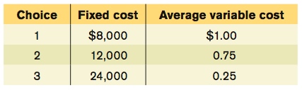
A. B. C. The accompanying table shows the average total cost of producing 12,000, 22,000, and 30,000 units for each of the three choices of fixed cost. For example, if the firm makes choice 1, the total cost of producing 12,000 units of output is $8,000 + 12,000 x $1.00 = $20,000. The average total cost of producing 12,000 units of output is therefore $20,000/12,000 = $1.67. The other average total costs are calculated similarly. So if the firm wanted to produce 12,000 units, it would make choice 1 because this gives it the lowest average total cost. If it wanted to produce 22,000 units, it would make choice 2. If it wanted to produce 30,000 units, it would make choice 3.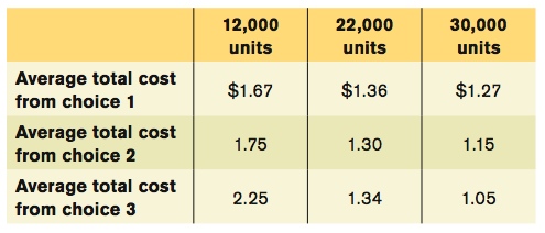
Question
The accompanying table shows three possible combinations of fixed cost and average variable cost. Average variable cost is constant in this example (it does not vary with the quantity of output produced). Suppose that the firm, which has historically produced 12,000 units, experiences a sharp, permanent increase in demand that leads it to produce 22,000 units. Which of the following explains how its average total cost will change in the short run and in the long run?
A. B. Having historically produced 12,000 units, the firm would have adopted choice 1. When producing 12,000 units, the firm would have had an average total cost of $1.67. When output jumps to 22,000 units, the firm cannot alter its choice of fixed cost in the short run, so its average total cost in the short run will be $1.36. In the long run, however, it will adopt choice 2, making its average total cost fall to $1.30.Question
The accompanying table shows three possible combinations of fixed cost and average variable cost. Average variable cost is constant in this example (it does not vary with the quantity of output produced). Suppose that the firm, which has historically produced 12,000 units, experiences a sharp, permanent increase in demand that leads it to produce 22,000 units. What should the firm do instead if it believes the change in demand is temporary?
A. B. If the firm believes that the increase in demand is temporary, it should not alter its fixed cost from choice 1 because choice 2 generates higher average total cost as soon as output falls back to its original quantity of 12,000 units: $1.75 versus $1.67.
- In each of the following cases, explain what kind of scale effects you think the firm will experience and why.
Question
In the following case, what kind of scale effects will the firm experience?
Case: A telemarketing firm in which employees make sales calls using computers and telephones.A. B. C. This firm is likely to experience constant returns to scale. To increase output, the firm must hire more workers, purchase more computers, and pay additional telephone charges. Because these inputs are easily available, their long-run average total cost is unlikely to change as output increases.Question
In the following case, what kind of scale effects will the firm experience?
Case: An interior design firm in which design projects are based on the expertise of the firm’s ownerA. B. C. This firm is likely to experience decreasing returns to scale. As the firm takes on more projects, the costs of communication and coordination required to implement the expertise of the firm’s owner are likely to increase.Question
In the following case, what kind of scale effects will the firm experience?
Case: A diamond mining companyA. B. C. This firm is likely to experience increasing returns to scale. Because diamond mining requires a large initial set-up cost for excavation equipment, long-run average total cost will fall as output increases.
Question
Draw a graph like Figure 6-12 and insert a short-run average total cost curve corresponding to a long-run output choice of 5 cases of salsa per day. Use the graph to show why Selena should change her fixed cost if she expects to produce only 4 cases per day for a long period of time.
Solutions appear at back of book.