Production and Profits
Consider Jennifer and Jason, who run an organic tomato farm. Suppose that the market price of organic tomatoes is $18 per bushel and that Jennifer and Jason are price-takers—they can sell as much as they like at that price. Then we can use the data in Table 7-1 to find their profit-maximizing level of output by direct calculation.
TABLE 7-1 Profit for Jennifer and Jason’s Farm When Market Price Is $18
| Quantity of tomatoes Q (bushels) | Total revenue TR | Total cost TC | Profit TR – TC |
|---|---|---|---|
| 0 | $0 | $14 | −$14 |
| 1 | 18 | 30 | −12 |
| 2 | 36 | 36 | 0 |
| 3 | 54 | 44 | 10 |
| 4 | 72 | 56 | 16 |
| 5 | 90 | 72 | 18 |
| 6 | 108 | 92 | 16 |
| 7 | 126 | 116 | 10 |
The first column shows the quantity of output in bushels, and the second column shows Jennifer and Jason’s total revenue from their output: the market value of their output. Total revenue, TR, is equal to the market price multiplied by the quantity of output:
(7-1) TR = P × Q
In this example, total revenue is equal to $18 per bushel times the quantity of output in bushels.
The third column of Table 7-1 shows Jennifer and Jason’s total cost. The fourth column shows their profit, equal to total revenue minus total cost:
(7-2) Profit = TR – TC
As indicated by the numbers in the table, profit is maximized at an output of 5 bushels, where profit is equal to $18. But we can gain more insight into the profit-maximizing choice of output by viewing it as a problem of marginal analysis, a task we’ll do next.
Using Marginal Analysis to Choose the Profit-Maximizing Quantity of Output
The marginal benefit of a good or service is the additional benefit derived from producing one more unit of that good or service.
The principle of marginal analysis says that the optimal amount of an activity is the quantity at which marginal benefit equals marginal cost.
Marginal revenue is the change in total revenue generated by an additional unit of output.
Recall from Chapter 6 the definition of marginal cost: the additional cost incurred by producing one more unit of that good or service. Similarly, the marginal benefit of a good or service is the additional benefit gained from producing one more unit of a good or service. We are now ready to use the principle of marginal analysis, which says that the optimal amount of an activity is the level at which marginal benefit is equal to marginal cost.
To apply this principle, consider the effect on a producer’s profit of increasing output by one unit. The marginal benefit of that unit is the additional revenue generated by selling it; this measure has a name—it is called the marginal revenue of that unit of output. The general formula for marginal revenue is:

or
MR = ΔTR/ΔQ
According to the optimal output rule, profit is maximized by producing the quantity of output at which the marginal revenue of the last unit produced is equal to its marginal cost.
So Jennifer and Jason maximize their profit by producing bushels up to the point at which the marginal revenue is equal to marginal cost. We can summarize this as the producer’s optimal output rule: profit is maximized by producing the quantity at which the marginal revenue of the last unit produced is equal to its marginal cost. That is, MR = MC at the optimal quantity of output.
We can learn how to apply the optimal output rule with the help of Table 7-2, which provides various short-run cost measures for Jennifer and Jason’s farm. The second column contains the farm’s variable cost, and the third column shows its total cost of output based on the assumption that the farm incurs a fixed cost of $14. The fourth column shows their marginal cost. Notice that, in this example, the marginal cost initially falls as output rises but then begins to increase. This gives the marginal cost curve the “swoosh” shape described in the Selena’s Gourmet Salsas example in Chapter 6. (Shortly it will become clear that this shape has important implications for short-run production decisions.)
TABLE 7-2 Short-Run Costs for Jennifer and Jason’s Farm
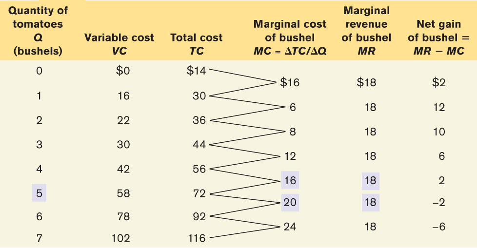
The fifth column contains the farm’s marginal revenue, which has an important feature: Jennifer and Jason’s marginal revenue is constant at $18 for every output level. The sixth and final column shows the calculation of the net gain per bushel of tomatoes, which is equal to marginal revenue minus marginal cost—or, equivalently in this case, market price minus marginal cost. As you can see, it is positive for the 1st through 5th bushels; producing each of these bushels raises Jennifer and Jason’s profit. For the 6th and 7th bushels, however, net gain is negative: producing them would decrease, not increase, profit. (You can verify this by examining Table 7-1.) So 5 bushels are Jennifer and Jason’s profit-maximizing output; it is the level of output at which marginal cost is equal to the market price, $18.
According to the price-taking firm’s optimal output rule, a price-taking firm’s profit is maximized by producing the quantity of output at which the market price is equal to the marginal cost of the last unit produced.
This example, in fact, illustrates another general rule derived from marginal analysis—the price-taking firm’s optimal output rule, which says that a price-taking firm’s profit is maximized by producing the quantity of output at which the market price is equal to the marginal cost of the last unit produced. That is, P = MC at the price-taking firm’s optimal quantity of output. In fact, the price-taking firm’s optimal output rule is just an application of the optimal output rule to the particular case of a price-taking firm. Why? Because in the case of a price-taking firm, marginal revenue is equal to the market price.
A price-taking firm cannot influence the market price by its actions. It always takes the market price as given because it cannot lower the market price by selling more or raise the market price by selling less. So, for a price-taking firm, the additional revenue generated by producing one more unit is always the market price. We will need to keep this fact in mind in future chapters, where we will learn that marginal revenue is not equal to the market price if the industry is not perfectly competitive. As a result, firms are not price-takers when an industry is not perfectly competitive.
The marginal revenue curve shows how marginal revenue varies as output varies.
For the remainder of this chapter, we will assume that the industry in question is like organic tomato farming, perfectly competitive. Figure 7-1 shows that Jennifer and Jason’s profit-maximizing quantity of output is, indeed, the number of bushels at which the marginal cost of production is equal to price. The figure shows the marginal cost curve, MC, drawn from the data in the fourth column of Table 7-2. We plot the marginal cost of increasing output from 1 to 2 bushels halfway between 1 and 2, and so on. The horizontal line at $18 is Jennifer and Jason’s marginal revenue curve.
FIGURE 7-1 The Price-Taking Firm’s Profit-Maximizing Quantity of Output

Note that whenever a firm is a price-taker, its marginal revenue curve is a horizontal line at the market price: it can sell as much as it likes at the market price. Regardless of whether it sells more or less, the market price is unaffected. In effect, the individual firm faces a horizontal, perfectly elastic demand curve for its output—an individual demand curve for its output that is equivalent to its marginal revenue curve. The marginal cost curve crosses the marginal revenue curve at point E. Sure enough, the quantity of output at E is 5 bushels.
Does this mean that the price-taking firm’s production decision can be entirely summed up as “produce up to the point where the marginal cost of production is equal to the price”? No, not quite. Before applying the profit-maximizing principle of marginal analysis to determine how much to produce, a potential producer must as a first step answer an “either–or” question: should it produce at all? If the answer to that question is yes, it then proceeds to the second step—a “how much” decision: maximizing profit by choosing the quantity of output at which marginal cost is equal to price.
What if Marginal Revenue and Marginal Cost Aren’T Exactly Equal?
The optimal output rule says that to maximize profit, you should produce the quantity at which marginal revenue is equal to marginal cost. But what do you do if there is no output level at which marginal revenue equals marginal cost? In that case, you produce the largest quantity for which marginal revenue exceeds marginal cost. This is the case in Table 7-2 at an output of 5 bushels. The simpler version of the optimal output rule applies when production involves large numbers, such as hundreds or thousands of units. In such cases marginal cost comes in small increments, and there is always a level of output at which marginal cost almost exactly equals marginal revenue.
To understand why the first step in the production decision involves an “either–or” question, we need to ask how we determine whether it is profitable or unprofitable to produce at all.
When Is Production Profitable?
Economic profit is equal to revenue minus the opportunity cost of resources used.
An explicit cost is a cost that requires an outlay of money.
An implicit cost does not require an outlay of money; it is measured by the value, in dollar terms, of benefits that are forgone.
Accounting profit is equal to revenue minus explicit cost. It is usually larger than economic profit.
A firm’s decision whether or not to stay in a given business depends on its economic profit—the firm’s revenue minus the opportunity cost of its resources. To put it in a slightly different way: in the calculation of economic profit, a firm’s total cost incorporates explicit cost and implicit cost. An explicit cost is a cost that involves actually laying out money. An implicit cost does not require an outlay of money; it is measured by the value, in dollar terms, of benefits that are forgone.
In contrast, accounting profit is profit calculated using only the explicit costs incurred by the firm. It is the firm’s revenue minus the explicit cost and depreciation. This means that economic profit incorporates the opportunity cost of resources owned by the firm and used in the production of output, while accounting profit does not.
A firm may make positive accounting profit while making zero or even negative economic profit. It’s important to understand clearly that a firm’s decision to produce or not, to stay in business or to close down permanently, should be based on economic profit, not accounting profit.
We will assume that the cost numbers given in Tables 7-1 and 7-2 include all costs, implicit as well as explicit, and that the profit numbers in Table 7-1 are therefore economic profit. So what determines whether Jennifer and Jason’s farm earns a profit or generates a loss? The answer is that, given the farm’s cost curves, whether or not it is profitable depends on the market price of tomatoes—specifically, whether the market price is more or less than the farm’s minimum average total cost.
In Table 7-3 we calculate short-run average variable cost and short-run average total cost for Jennifer and Jason’s farm. These are short-run values because we take fixed cost as given. (We’ll turn to the effects of changing fixed cost shortly.) The short-run average total cost curve, ATC, is shown in Figure 7-2, along with the marginal cost curve, MC, from Figure 7-1. As you can see, average total cost is minimized at point C, corresponding to an output of 4 bushels—the minimum-cost output—and an average total cost of $14 per bushel.
TABLE 7-3 Short-Run Average Costs for Jennifer and Jason’s Farm
| Quantity of tomatoes Q (bushels) | Variable cost VC | Total cost TC | Short-run average variable cost of bushel AVC = VC/Q | Short-run average total cost of bushel ATC = TC/Q |
|---|---|---|---|---|
| 1 | $16.00 | $30.00 | $16.00 | $30.00 |
| 2 | 22.00 | 36.00 | 11.00 | 18.00 |
| 3 | 30.00 | 44.00 | 10.00 | 14.67 |
| 4 | 42.00 | 56.00 | 10.50 | 14.00 |
| 5 | 58.00 | 72.00 | 11.60 | 14.40 |
| 6 | 78.00 | 92.00 | 13.00 | 15.33 |
| 7 | 102.00 | 116.00 | 14.57 | 16.57 |
FIGURE 7-2 Costs and Production in the Short Run

To see how these curves can be used to decide whether production is profitable or unprofitable, recall that profit is equal to total revenue minus total cost, TR – TC. This means:
- If the firm produces a quantity at which TR > TC, the firm is profitable.
- If the firm produces a quantity at which TR = TC, the firm breaks even.
- If the firm produces a quantity at which TR < TC, the firm incurs a loss.
We can also express this idea in terms of revenue and cost per unit of output. If we divide profit by the number of units of output, Q, we obtain the following expression for profit per unit of output:
(7-4) Profit/Q = TR/Q − TC/Q
TR/Q is average revenue, which is the market price. TC/Q is average total cost. So a firm is profitable if the market price for its product is more than the average total cost of the quantity the firm produces; a firm loses money if the market price is less than average total cost of the quantity the firm produces. This means:
- If the firm produces a quantity at which P > ATC, the firm is profitable.
- If the firm produces a quantity at which P = ATC, the firm breaks even.
- If the firm produces a quantity at which P < ATC, the firm incurs a loss.
Figure 7-3 illustrates this result, showing how the market price determines whether a firm is profitable. It also shows how profits are depicted graphically. Each panel shows the marginal cost curve, MC, and the short-run average total cost curve, ATC. Average total cost is minimized at point C. Panel (a) shows the case we have already analyzed, in which the market price of tomatoes is $18 per bushel. Panel (b) shows the case in which the market price of tomatoes is lower, $10 per bushel.
FIGURE 7-3 Profitability and the Market Price

In panel (a), we see that at a price of $18 per bushel the profit-maximizing quantity of output is 5 bushels, indicated by point E, where the marginal cost curve, MC, intersects the marginal revenue curve—which for a price-taking firm is a horizontal line at the market price. At that quantity of output, average total cost is $14.40 per bushel, indicated by point Z. Since the price per bushel exceeds average total cost per bushel, Jennifer and Jason’s farm is profitable.
Jennifer and Jason’s total profit when the market price is $18 is represented by the area of the shaded rectangle in panel (a). To see why, notice that total profit can be expressed in terms of profit per unit:
(7-5) Profit = TR − TC = (TR/Q – TC/Q) × Q
or, equivalently,
Profit = (P – ATC) × Q
since P is equal to TR/Q and ATC is equal to TC/Q. The height of the shaded rectangle in panel (a) corresponds to the vertical distance between points E and Z. It is equal to P − ATC = $18.00 – $14.40 = $3.60 per bushel. The shaded rectangle has a width equal to the output: Q = 5 bushels. So the area of that rectangle is equal to Jennifer and Jason’s profit: 5 bushels × $3.60 profit per bushel = $18—the same number we calculated in Table 7-1.
What about the situation illustrated in panel (b)? Here the market price of tomatoes is $10 per bushel. Setting price equal to marginal cost leads to a profit-maximizing output of 3 bushels, indicated by point A. At this output, Jennifer and Jason have an average total cost of $14.67 per bushel, indicated by point Y. At their profit-maximizing output quantity—3 bushels—average total cost exceeds the market price. This means that Jennifer and Jason’s farm generates a loss, not a profit.
How much do they lose by producing when the market price is $10? On each bushel they lose ATC − P = $14.67 – $10.00 = $4.67, an amount corresponding to the vertical distance between points A and Y. And they would produce 3 bushels, which corresponds to the width of the shaded rectangle. So the total value of the losses is $4.67 × 3 = $14.00 (adjusted for rounding error), an amount that corresponds to the area of the shaded rectangle in panel (b).
But how does a producer know, in general, whether or not its business will be profitable? It turns out that the crucial test lies in a comparison of the market price to the producer’s minimum average total cost. On Jennifer and Jason’s farm, minimum average total cost, which is equal to $14, occurs at an output quantity of 4 bushels, indicated by point C. Whenever the market price exceeds minimum average total cost, the producer can find some output level for which the average total cost is less than the market price. In other words, the producer can find a level of output at which the firm makes a profit. So Jennifer and Jason’s farm will be profitable whenever the market price exceeds $14. And they will achieve the highest possible profit by producing the quantity at which marginal cost equals the market price.
Conversely, if the market price is less than minimum average total cost, there is no output level at which price exceeds average total cost. As a result, the firm will be unprofitable at any quantity of output. As we saw, at a price of $10—an amount less than minimum average total cost—Jennifer and Jason did indeed lose money. By producing the quantity at which marginal cost equals the market price, Jennifer and Jason did the best they could, but the best that they could do was a loss of $14. Any other quantity would have increased the size of their loss.
The break-even price of a price-taking firm is the market price at which it earns zero profit.
The minimum average total cost of a price-taking firm is called its break-even price, the price at which it earns zero profit. (Recall that’s economic profit.) A firm will earn positive profit when the market price is above the break-even price, and it will suffer losses when the market price is below the break-even price. Jennifer and Jason’s break-even price of $14 is the price at point C in Figures 7-2 and 7-3.
So the rule for determining whether a producer of a good is profitable depends on a comparison of the market price of the good to the producer’s break-even price—its minimum average total cost:
- Whenever the market price exceeds minimum average total cost, the producer is profitable.
- Whenever the market price equals minimum average total cost, the producer breaks even.
- Whenever the market price is less than minimum average total cost, the producer is unprofitable.
The Short-Run Production Decision
You might be tempted to say that if a firm is unprofitable because the market price is below its minimum average total cost, it shouldn’t produce any output. In the short run, however, this conclusion isn’t right. In the short run, sometimes the firm should produce even if price falls below minimum average total cost. The reason is that total cost includes fixed cost—cost that does not depend on the amount of output produced and can only be altered in the long run. In the short run, fixed cost must still be paid, regardless of whether or not a firm produces. For example, if Jennifer and Jason have rented a tractor for the year, they have to pay the rent on the tractor regardless of whether they produce any tomatoes. Since it cannot be changed in the short run, their fixed cost is irrelevant to their decision about whether to produce or shut down in the short run.
Although fixed cost should play no role in the decision about whether to produce in the short run, other costs—variable costs—do matter. An example of variable costs is the wages of workers who must be hired to help with planting and harvesting. Variable costs can be saved by not producing; so they should play a role in determining whether or not to produce in the short run.
Let’s turn to Figure 7-4: it shows both the short-run average total cost curve, ATC, and the short-run average variable cost curve, AVC, drawn from the information in Table 7-3. Recall that the difference between the two curves—the vertical distance between them—represents average fixed cost, the fixed cost per unit of output, FC/Q. Because the marginal cost curve has a “swoosh” shape—falling at first before rising—the short-run average variable cost curve is U-shaped: the initial fall in marginal cost causes average variable cost to fall as well, before rising marginal cost eventually pulls it up again. The short-run average variable cost curve reaches its minimum value of $10 at point A, at an output of 3 bushels.
FIGURE 7-4 The Short-Run Individual Supply Curve

We are now prepared to fully analyze the optimal production decision in the short run. We need to consider two cases:
- When the market price is below minimum average variable cost
- When the market price is greater than or equal to minimum average variable cost
A firm will cease production in the short run if the market price falls below the shut-down price, which is equal to minimum average variable cost.
When the market price is below minimum average variable cost, the price the firm receives per unit is not covering its variable cost per unit. A firm in this situation should cease production immediately. Why? Because there is no level of output at which the firm’s total revenue covers its variable costs—the costs it can avoid by not operating. In this case the firm maximizes its profits by not producing at all—by, in effect, minimizing its losses. It will still incur a fixed cost in the short run, but it will no longer incur any variable cost. This means that the minimum average variable cost is equal to the shut-down price, the price at which the firm ceases production in the short run.
When price is greater than minimum average variable cost, however, the firm should produce in the short run. In this case, the firm maximizes profit—or minimizes loss—by choosing the output quantity at which its marginal cost is equal to the market price. For example, if the market price of tomatoes is $18 per bushel, Jennifer and Jason should produce at point E in Figure 7-4, corresponding to an output of 5 bushels. Note that point C in Figure 7-4 corresponds to the farm’s break-even price of $14 per bushel. Since E lies above C, Jennifer and Jason’s farm will be profitable; they will generate a per-bushel profit of $18.00 – $14.40 = $3.60 when the market price is $18.
But what if the market price lies between the shut-down price and the break-even price—that is, between minimum average variable cost and minimum average total cost? In the case of Jennifer and Jason’s farm, this corresponds to prices anywhere between $10 and $14—say, a market price of $12. At $12, Jennifer and Jason’s farm is not profitable; since the market price is below minimum average total cost, the farm is losing the difference between price and average total cost per unit produced. Yet even if it isn’t covering its total cost per unit, it is covering its variable cost per unit and some—but not all—of the fixed cost per unit. If a firm in this situation shuts down, it would incur no variable cost but would incur the full fixed cost. As a result, shutting down generates an even greater loss than continuing to operate.
This means that whenever price lies between minimum average total cost and minimum average variable cost, the firm is better off producing some output in the short run. The reason is that by producing, it can cover its variable cost per unit and at least some of its fixed cost, even though it is incurring a loss. In this case, the firm maximizes profit—that is, minimizes loss—by choosing the quantity of output at which its marginal cost is equal to the market price. So if Jennifer and Jason face a market price of $12 per bushel, their profit-maximizing output is given by point B in Figure 7-4, corresponding to an output of 3.5 bushels.
A sunk cost is a cost that has already been incurred and is nonrecoverable. A sunk cost should be ignored in decisions about future actions.
It’s worth noting that the decision to produce when the firm is covering its variable costs but not all of its fixed cost is similar to the decision to ignore sunk costs. A sunk cost is a cost that has already been incurred and cannot be recouped; and because it cannot be changed, it should have no effect on any current decision. In the short-run production decision, fixed cost is, in effect, like a sunk cost—it has been spent, and it can’t be recovered in the short run. This comparison also illustrates why variable cost does indeed matter in the short run: it can be avoided by not producing.
And what happens if market price is exactly equal to the shut-down price, minimum average variable cost? In this instance, the firm is indifferent between producing 3 units or 0 units. As we’ll see shortly, this is an important point when looking at the behavior of an industry as a whole. For the sake of clarity, we’ll assume that the firm, although indifferent, does indeed produce output when price is equal to the shut-down price.
The short-run individual supply curve shows how an individual producer’s profit-maximizing output quantity depends on the market price, taking fixed cost as given.
Putting everything together, we can now draw the short-run individual supply curve of Jennifer and Jason’s farm, the red line in Figure 7-4; it shows how the profit-maximizing quantity of output in the short run depends on the price. As you can see, the curve is in two segments. The upward-sloping red segment starting at point A shows the short-run profit-maximizing output when market price is equal to or above the shut-down price of $10 per bushel.
As long as the market price is equal to or above the shut-down price, Jennifer and Jason produce the quantity of output at which marginal cost is equal to the market price. That is, at market prices equal to or above the shut-down price, the firm’s short-run supply curve corresponds to its marginal cost curve. But at any market price below minimum average variable cost—in this case, $10 per bushel—the firm shuts down and output drops to zero in the short run. This corresponds to the vertical segment of the curve that lies on top of the vertical axis.
Do firms really shut down temporarily without going out of business? Yes. In fact, in some businesses temporary shut-downs are routine. The most common examples are industries in which demand is highly seasonal, like outdoor amusement parks in climates with cold winters. Such parks would have to offer very low prices to entice customers during the colder months—prices so low that the owners would not cover their variable costs (principally wages and electricity). The wiser choice economically is to shut down until warm weather brings enough customers who are willing to pay a higher price.
Changing Fixed Cost
Although fixed cost cannot be altered in the short run, in the long run firms can acquire or get rid of machines, buildings, and so on. As we learned in Chapter 6, in the long run the level of fixed cost is a matter of choice. There we saw that a firm will choose the level of fixed cost that minimizes the average total cost for its desired output quantity. Now we will focus on an even bigger question facing a firm when choosing its fixed cost: whether to incur any fixed cost at all by remaining in its current business.
In the long run, a producer can always eliminate fixed cost by selling off its plant and equipment. If it does so, of course, it can’t ever produce—it has exited the industry. In contrast, a potential producer can take on some fixed cost by acquiring machines and other resources, which puts it in a position to produce—it can enter the industry. In most perfectly competitive industries the set of producers, although fixed in the short run, changes in the long run as firms enter or exit the industry.
Consider Jennifer and Jason’s farm once again. In order to simplify our analysis, we will sidestep the problem of choosing among several possible levels of fixed cost. Instead, we will assume from now on that Jennifer and Jason have only one possible choice of fixed cost if they operate, the amount of $14 that was the basis for the calculations in Tables 7-1, 7-2, and 7-3. (With this assumption, Jennifer and Jason’s short-run average total cost curve and long-run average total cost curve are one and the same.) Alternatively, they can choose a fixed cost of zero if they exit the industry.
Suppose that the market price of organic tomatoes is consistently less than $14 over an extended period of time. In that case, Jennifer and Jason never fully cover their fixed cost: their business runs at a persistent loss. In the long run, then, they can do better by closing their business and leaving the industry. In other words, in the long run firms will exit an industry if the market price is consistently less than their break-even price—their minimum average total cost.
Conversely, suppose that the price of organic tomatoes is consistently above the break-even price, $14, for an extended period of time. Because their farm is profitable, Jennifer and Jason will remain in the industry and continue producing.
But things won’t stop there. The organic tomato industry meets the criterion of free entry: there are many potential organic tomato producers because the necessary inputs are easy to obtain. And the cost curves of those potential producers are likely to be similar to those of Jennifer and Jason, since the technology used by other producers is likely to be very similar to that used by Jennifer and Jason. If the price is high enough to generate profits for existing producers, it will also attract some of these potential producers into the industry. So in the long run a price in excess of $14 should lead to entry: new producers will come into the organic tomato industry.
As we will see in the next section, exit and entry lead to an important distinction between the short-run industry supply curve and the long-run industry supply curve.
Summing Up: The Perfectly Competitive Firm’s Profitability and Production Conditions
In this chapter, we’ve studied where the supply curve for a perfectly competitive, price-taking firm comes from. Every perfectly competitive firm makes its production decisions by maximizing profit, and these decisions determine the supply curve. Table 7-4 summarizes the perfectly competitive firm’s profitability and production conditions. It also relates them to entry into and exit from the industry.
TABLE 7-4 Summary of the Perfectly Competitive Firm’s Profitability and Production Conditions
| Profitability condition(minimum ATC = break–even price) | Result |
|---|---|
| P > minimum ATC | Firm profitable. Entry into industry in the long run. |
| P = minimum ATC | Firm breaks even. No entry into or exit from industry in the long run. |
| P < minimum ATC | Firm unprofitable. Exit from industry in the long run. |
| Production condition (minimum AVC = shut–down price) | Result |
| P > minimum AVC | Firm produces in the short run. If P < minimum ATC, firm covers variable cost and some but not all of fixed cost. If P > minimum ATC, firm covers all variable cost and fixed cost. |
| P = minimum AVC | Firm indifferent between producing in the short run or not. Just covers variable cost. |
| P < minimum AVC | Firm shuts down in the short run. Does not cover variable cost. |
Prices are Up … But So Are Costs
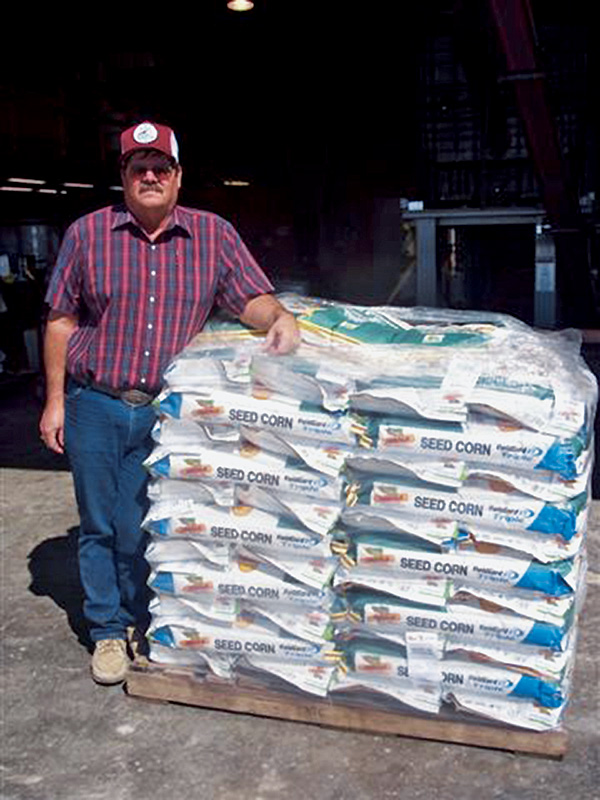
Because of the Energy Policy Act of 2005, 7.5 billion gallons of alternative fuel, mostly corn-based ethanol, was added to the American fuel supply to help reduce gasoline consumption. The unsurprising result of this mandate: the demand for corn skyrocketed, along with the price. In August 2012, a bushel of corn hit a high of $8.32, nearly quadruple the early January 2005 price of $2.09.
This sharp rise in the price of corn caught the eye of American farmers like Ronnie Gerik of Aquilla, Texas, who reduced the size of his cotton crop and increased his corn acreage by 40%. Overall, the U.S. corn acreage planted in 2011 was 9% more than the average planted over the previous decade, and 4% more corn was planted in 2012 than in 2011. Like Gerik, other farmers substituted corn production for the production of other crops; for example, in 2011, soybean acreage was down around 3% and decreased by another 1% in 2012.
Quick Review
- Per the principle of marginal analysis, the optimal amount of an activity is the quantity at which marginal benefit equals marginal cost.
- A producer chooses output according to the optimal output rule. For a price-taking firm, marginal revenue is equal to price and it chooses output according to the price-taking firm’s optimal output rule.
- The economic profit of a company includes explicit costs and implicit costs. It isn’t necessarily equal to the accounting profit.
- A firm is profitable whenever price exceeds its break-even price, equal to its minimum average total cost. Below that price it is unprofitable. It breaks even when price is equal to its break-even price.
- Fixed cost is irrelevant to the firm’s optimal short-run production decision. When price exceeds its shut-down price, minimum average variable cost, the price-taking firm produces the quantity of output at which marginal cost equals price. When price is lower than its shut-down price, it ceases production. Like sunk costs, fixed costs are irrelevant to the firm’s short-run production decisions. These decisions define the firm’s short-run individual supply curve.
- Over time, fixed cost matters. If price consistently falls below minimum average total cost, a firm will exit the industry. If price exceeds minimum average total cost, the firm is profitable and will remain in the industry; other firms will enter the industry in the long run.
Although this sounds like a sure way to make a profit, Gerik and farmers like him were taking a gamble. Consider the cost of an important input, fertilizer. Corn requires more fertilizer than other crops, and with more farmers planting corn, the increased demand for fertilizer led to a price increase. Prices for fertilizer produced from nitrogen nearly doubled from 2005 to 2012. Moreover, corn is more sensitive to the amount of rainfall than a crop like cotton. So farmers who plant corn in drought-prone places like Texas are increasing their risk of loss. Gerik had to incorporate into his calculations his best guess of what a dry spell would cost him.
Despite all this, what Gerik and other farmers did made complete economic sense. By planting more corn, each one moved up his or her individual short-run supply curve for corn production. And because the individual supply curve is the marginal cost curve, each farmer’s costs also went up because of the need to apply more inputs—inputs that are now more expensive to obtain.
So the moral of the story is that farmers will increase their corn acreage until the marginal cost of producing corn is approximately equal to the market price of corn, which shouldn’t come as a surprise because corn production satisfies all the requirements of a perfectly competitive industry.
Check Your Understanding 7-2
Question
Draw a short-run diagram showing a U-shaped average total cost curve, a U-shaped average variable cost curve, and a "swoosh"-shaped marginal cost curve. When is the following action optimal?
Action: The firm shuts down immediately.A. B. C. The firm should shut down immediately when price is less than minimum average variable cost, the shut-down price. In the accompanying diagram, this is optimal for prices in the range 0 to P1.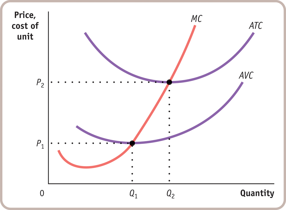
Question
Draw a short-run diagram showing a U-shaped average total cost curve, a U-shaped average variable cost curve, and a "swoosh"-shaped marginal cost curve. When is the following action optimal?
Action: The firm operates in the short run despite sustaining a loss.A. B. C. When price is greater than minimum average variable cost (the shut-down price) but less than minimum average total cost (the break-even price), the firm should continue to operate in the short-run even though it is making a loss. This is optimal for prices in the range P1 to P2 and for quantities Q1 to Q2.Question
Draw a short-run diagram showing a U-shaped average total cost curve, a U-shaped average variable cost curve, and a "swoosh"-shaped marginal cost curve. When is the following action optimal?
Action: The firm operates while making a profit.A. B. C. When price exceeds minimum average total cost (the break-even price), the firm makes a profit. This happens for prices in excess of P2 and results in quantities greater than Q2.
Question
The state of Maine has a very active lobster industry, which harvests lobsters during the summer months. During the rest of the year, lobsters can be obtained from other parts of the world but at a much higher price. Maine is also full of “lobster shacks,” roadside restaurants serving lobster dishes that are open only during the summer. Which of the following explains why it is optimal for lobster shacks to operate only during the summer?
A. B. This is an example of a temporary shut-down by a firm when the market price lies below the shut-down price, the minimum average variable cost. In this case, the market price is the price of a lobster meal and variable cost is the variable cost of serving such a meal, such as the cost of the lobster, employee wages, and so on. In this example, however, it is the average variable cost curve rather than the market price that shifts over time, due to seasonal changes in the cost of lobsters. Maine lobster shacks have relatively low average variable cost during the summer, when cheap Maine lobsters are available; during the rest of the year, their average variable cost is relatively high due to the high cost of imported lobsters. So the lobster shacks are open for business during the summer, when their minimum average variable cost lies below price; but they close during the rest of the year, when price lies below their minimum average variable cost.
Solutions appear at back of book.