Matching Up Savings and Investment Spending
We learned in the previous chapter that two of the essential ingredients in economic growth are increases in the economy’s levels of human capital and physical capital. Human capital is largely provided by governments through public education. (In countries with a large private education sector, like the United States, private post-
Who pays for private investment spending? In some cases it’s the people or corporations that actually do the spending—
To understand how investment spending is financed, we need to look first at how savings and investment spending are related for the economy as a whole. Then we will examine how savings are allocated among investment spending projects.
The Savings–Investment Spending Identity
According to the savings–
The most basic point to understand about savings and investment spending is that they are always equal. This is not a theory; it’s a fact of accounting called the savings–
To see why the savings–

where C is spending by consumers, I is investment spending, G is government purchases of goods and services, X is the value of exports to other countries, and IM is spending on imports from other countries.
The Savings–Investment Spending Identity in a Closed Economy
PITFALLS: INVESTMENT VERSUS INVESTMENT SPENDING
INVESTMENT VERSUS INVESTMENT SPENDING
When macroeconomists use the term investment spending, they almost always mean “spending on new physical capital.” This can be confusing, because in ordinary life we often say that someone who buys stocks or purchases an existing building is “investing.” The important point to keep in mind is that only spending that adds to the economy’s stock of physical capital is “investment spending.” In contrast, the act of purchasing an asset such as a share of stock, a bond, or existing real estate is “making an investment.”
In a closed economy, there are no exports or imports. So X = 0 and IM = 0, which makes Equation 10-

Now, what can be done with income? It can either be spent on consumption—

where S is savings. Meanwhile, as Equation 10-

Putting Equations 10-
Subtract consumption spending (C + G) from both sides, and we get:
As we said, then, it’s a basic accounting fact that savings equals investment spending for the economy as a whole.
The budget surplus is the difference between tax revenue and government spending when tax revenue exceeds government spending.
Now, let’s take a closer look at savings. Households are not the only parties that can save in an economy. In any given year, the government can save, too, if it collects more tax revenue than it spends. When this occurs, the difference is called a budget surplus and is equivalent to savings by government. If, alternatively, government spending exceeds tax revenue, there is a budget deficit—a negative budget surplus. In this case, we often say that the government is “dissaving”: by spending more than its tax revenues, the government is engaged in the opposite of savings.
The budget deficit is the difference between tax revenue and government spending when government spending exceeds tax revenue.
We’ll define the term budget balance to refer to both cases, with the understanding that the budget balance can be positive (a budget surplus) or negative (a budget deficit). The budget balance is defined as:
The budget balance is the difference between tax revenue and government spending.

Where T is the value of tax revenues and TR is the value of government transfers. The budget balance is equivalent to savings by government—
National savings, the sum of private savings and the budget balance, is the total amount of savings generated within the economy.

So Equations 10-
The Savings–
Net capital inflow is the total inflow of funds into a country minus the total outflow of funds out of a country.
The net effect of international inflows and outflows of funds on the total savings available for investment spending in any given country is known as the net capital inflow into that country, equal to the total inflow of foreign funds minus the total outflow of domestic funds to other countries. Like the budget balance, a net capital inflow can be negative—
PITFALLS: THE DIFFERENT KINDS OF CAPITAL
THE DIFFERENT KINDS OF CAPITAL
It’s important to understand clearly the three different kinds of capital: physical capital, human capital, and financial capital (as explained in the previous chapter):
Physical capital consists of manufactured resources such as buildings and machines.
Human capital is the improvement in the labor force generated by education and knowledge.
Financial capital is funds from savings that are available for investment spending. A country that has a positive net capital inflow is experiencing a flow of funds into the country from abroad that can be used for investment spending.
It’s important to note that, from a national perspective, a dollar generated by national savings and a dollar generated by capital inflow are not equivalent. Yes, they can both finance the same dollar’s worth of investment spending. But any dollar borrowed from a saver must eventually be repaid with interest. A dollar that comes from national savings is repaid with interest to someone domestically—
The fact that a net capital inflow represents funds borrowed from foreigners is an important aspect of the savings–

Rearranging Equation 10-

Using Equations 10-

So the application of the savings–
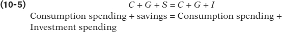
In the United States in 2013, investment spending totaled $3,244.3 billion. Private savings totaled $3,402 billion, offset by government savings of −$368 billion and supplemented by a net capital inflow of $423 billion. Notice that these numbers don’t quite add up; because data collection isn’t perfect, there is a “statistical discrepancy” of −$212 billion. But we know that this is an error in the data, not in the theory, because the savings–
Figure 10-1 shows what the savings–
10-1
The Savings–
The economy’s savings finance its investment spending. But how are these funds that are available for investment spending allocated among various projects? That is, what determines which projects get financed (such as Facebook’s server farms) and which don’t (such as Microsoft’s Courier tablet computer, an innovative concept that the software giant decided not to pursue)? We’ll see shortly that funds get allocated to investment spending projects using a familiar method: by the market, via supply and demand.
Who Enforces the Accounting?
The savings–
The short answer is that actual and desired investment spending aren’t always equal. Suppose that households suddenly decide to save more by spending less—
A real-
Of course, businesses respond to changes in their inventories by changing their production. The inventory reduction in late 2001 prepared the ground for a spurt in output in early 2002. We’ll examine the special role of inventories in economic fluctuations in Chapter 11.
The Market for Loanable Funds
For the economy as a whole, savings always equals investment spending. In a closed economy, savings is equal to national savings. In an open economy, savings is equal to national savings plus capital inflow. At any given time, however, savers, the people with funds to lend, are usually not the same as borrowers, the people who want to borrow to finance their investment spending. How are savers and borrowers brought together?
Savers and borrowers are matched up with one another in much the same way producers and consumers are matched up: through markets governed by supply and demand. In Figure 7-1, the expanded circular-
The loanable funds market is a hypothetical market that illustrates the market outcome of the demand for funds generated by borrowers and the supply of funds provided by lenders.
To do this, it helps to consider a somewhat simplified version of reality. As we noted in Chapter 7, there are a large number of different financial markets in the financial system, such as the bond market and the stock market. However, economists often work with a simplified model in which they assume that there is just one market that brings together those who want to lend money (savers) and those who want to borrow (firms with investment spending projects). This hypothetical market is known as the loanable funds market. The price that is determined in the loanable funds market is the interest rate, denoted by r. As we noted in Chapter 8, loans typically specify a nominal interest rate. So although we call r “the interest rate,” it is with the understanding that r is a nominal interest rate—
We’re not quite done simplifying things. There are, in reality, many different kinds of interest rates, because there are many different kinds of loans—
OK, now we’re ready to analyze how savings and investment get matched up.
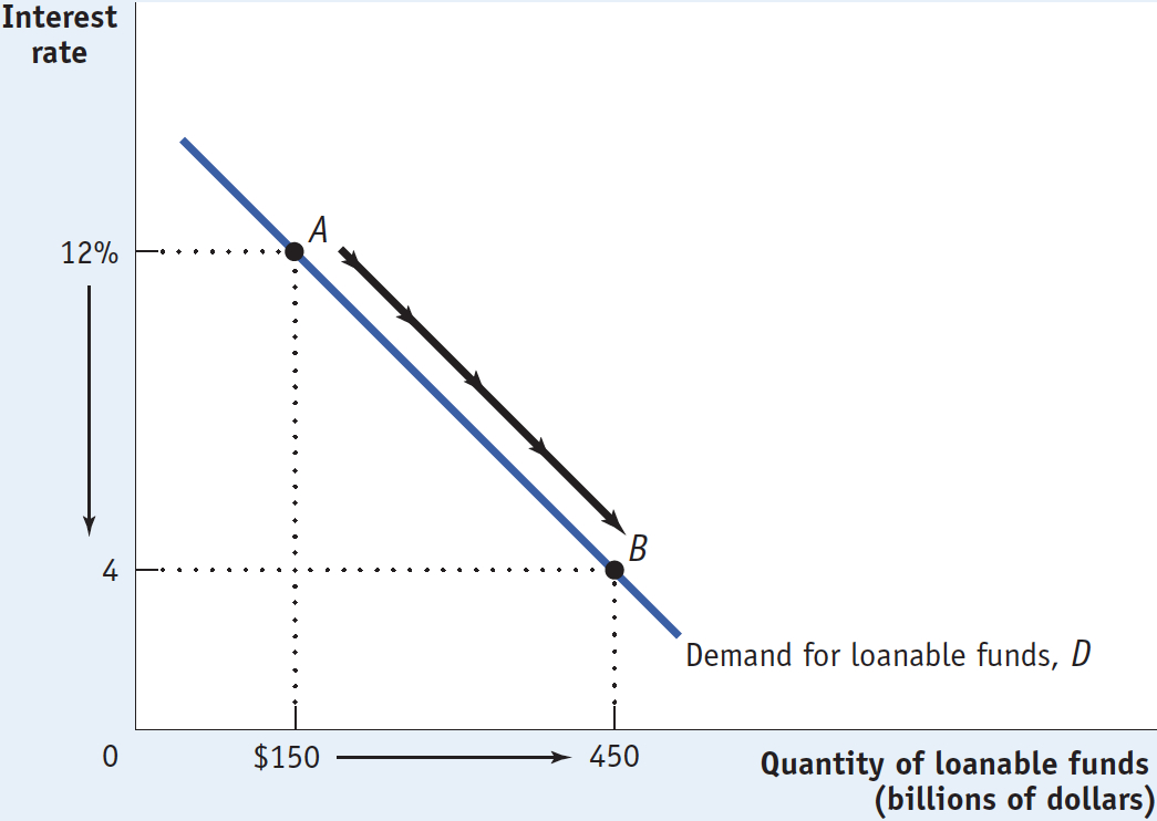
The Demand for Loanable Funds Figure 10-2 illustrates a hypothetical demand curve for loanable funds, D, which slopes downward. On the horizontal axis we show the quantity of loanable funds demanded. On the vertical axis we show the interest rate, which is the “price” of borrowing. But why does the demand curve for loanable funds slope downward?
10-2
The Demand for Loanable Funds
To answer this question, consider what a firm is doing when it engages in investment spending—
To answer that, we need to take into account the present value of the future return the firm expects to get. We examine the concept of present value in the accompanying For Inquiring Minds. Then, in the chapter’s appendix, we show how the concept of present value can be applied to dollars earned multiple years in the future. The appendix also addresses how present value is used to calculate the prices of shares of stock and bonds.
In present value calculations, we use the interest rate to determine how the value of a dollar in the future compares to the value of a dollar today. But the fact is that future dollars are worth less than a dollar today, and they are worth even less when the interest rate is higher.
Using Present Value
An understanding of the concept of present value shows why the demand curve for loanable funds slopes downward. A simple way to grasp the essence of present value is to consider an example that illustrates the difference in value between having a sum of money today and having the same sum of money a year from now.
Suppose that exactly one year from today you will graduate, and you want to reward yourself by taking a trip that will cost $1,000. In order to have $1,000 a year from now, how much do you need today? It’s not $1,000, and the reason why has to do with the interest rate. Let’s call the amount you need today X. We’ll use r to represent the interest rate you receive on funds deposited in the bank. If you put X into the bank today and earn interest rate r on it, then after one year, the bank will pay you X × (1 + r). If what the bank will pay you a year from now is equal to $1,000, then the amount you need today is
X × (1 + r) = $1,000
You can apply some basic algebra to find that
X = $1,000/(1 + r)
The present value of X is the amount of money needed today in order to receive X at a future date given the interest rate.
Notice that the value of X depends on the interest rate r, which is always greater than 0. This fact implies that X is always less than $1,000. For example, if r = 5% (that is, r = 0.05), then X = $952.38. In other words, having $952.38 today is equivalent to having $1,000 a year from now when the interest rate is 5%. That is, $952.38 is the value of $1,000 today given an interest rate of 5%. Now we can define the present value of X: it is the amount of money needed today in order to receive X in the future given the interest rate. In this numerical example, $952.38 is the present value of $1,000 received one year from now given an interest rate of 5%.

The concept of present value also applies to decisions made by firms. Think about a firm that has two potential investment projects in mind, each of which will yield $1,000 a year from now. However, each project has different initial costs—
The answer depends on the interest rate, which determines the present value of $1,000 a year from now. If the interest rate is 10%, the present value of $1,000 delivered a year from now is $909. In other words, at an interest rate of 10%, a $909 loan requires a repayment of $1,000 in a year’s time. A loan less than $909 requires a repayment less than $1,000, while a loan of more than $909 requires a repayment of more than $1,000. So only the first project, which has an initial cost of less than $909, is profitable, because its return in a year’s time is more than the amount of the loan repayment.
With an interest rate of 10%, the return on any project costing more than $909 is less than the amount the firm has to repay on its loan and is therefore unprofitable. If the interest rate is only 5%, however, the present value of $1,000 rises to $952. At this interest rate, both projects are profitable, because $952 exceeds both projects’ initial cost. So a firm will borrow more and engage in more investment spending when the interest rate is lower.
Meanwhile, similar calculations will be taking place at other firms. So a lower interest rate will lead to higher investment spending in the economy as a whole: the demand curve for loanable funds slopes downward.
The intuition behind present value calculations is simple. The interest rate measures the opportunity cost of investment spending that results in a future return: instead of spending money on an investment spending project, a company could simply put the money into the bank and earn interest on it. And the higher the interest rate, the more attractive it is to simply put money into the bank and let it earn interest instead of investing it in an investment spending project.
In other words, the higher the interest rate, the higher the opportunity cost of investment spending. And, the higher the opportunity cost of investment spending, the lower the number of investment spending projects firms want to carry out, and therefore the lower the quantity of loanable funds demanded. It is this insight (discussed in the accompanying For Inquiring Minds) that explains why the demand curve for loanable funds is downward sloping.
When businesses engage in investment spending, they spend money right now in return for an expected payoff in the future. To evaluate whether a particular investment spending project is worth undertaking, a business must compare the present value of the future payoff with the current cost of that project. If the present value of the future payoff is greater than the current cost, a project is profitable and worth investing in. If the interest rate falls, then the present value of any given project rises, so more projects pass that test. If the interest rate rises, then the present value of any given project falls, and fewer projects pass that test.
So total investment spending, and hence the demand for loanable funds to finance that spending, is negatively related to the interest rate. Thus, the demand curve for loanable funds slopes downward. You can see this in Figure 10-2. When the interest rate falls from 12% to 4%, the quantity of loanable funds demanded rises from $150 billion (point A) to $450 billion (point B).
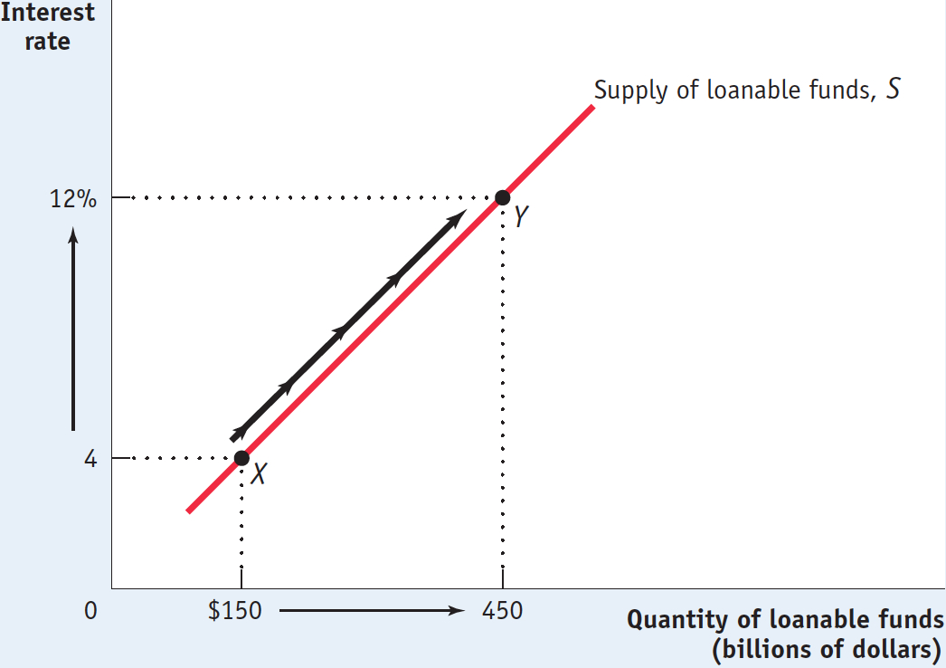
The Supply of Loanable Funds Figure 10-3 shows a hypothetical supply curve for loanable funds, S. Again, the interest rate plays the same role that the price plays in ordinary supply and demand analysis. But why is this curve upward sloping?
10-3
The Supply of Loanable Funds
The answer is that loanable funds are supplied by savers, and savers incur an opportunity cost when they lend to a business: the funds could instead be spent on consumption—
As a result, our hypothetical supply curve of loanable funds slopes upward. In Figure 10-3, lenders will supply $150 billion to the loanable funds market at an interest rate of 4% (point X); if the interest rate rises to 12%, the quantity of loanable funds supplied will rise to $450 billion (point Y).
The interest rate at which the quantity of loanable funds supplied equals the quantity of loanable funds demanded is the equilibrium interest rate.
The Equilibrium Interest Rate The interest rate at which the quantity of loanable funds supplied equals the quantity of loanable funds demanded is called the equilibrium interest rate. As you can see in Figure 10-4, the equilibrium interest rate, r*, and the total quantity of lending, Q*, are determined by the intersection of the supply and demand curves, at point E. Here, the equilibrium interest rate is 8%, at which $300 billion is lent and borrowed. In this equilibrium, only investment spending projects that are profitable if the interest rate is 8% or higher are funded. Projects that would not be undertaken unless they are profitable only when the interest rate falls below 8% are not funded. Correspondingly, only lenders who are willing to accept an interest rate of 8% or less will have their offers to lend funds accepted; lenders who demand an interest rate higher than 8% do not have their offers to lend accepted.
10-4
Equilibrium in the Loanable Funds Market
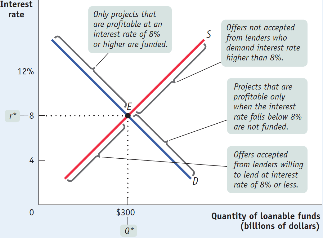
Figure 10-4 shows how the market for loanable funds matches up desired savings with desired investment spending: in equilibrium, the quantity of funds that savers want to lend is equal to the quantity of funds that firms want to borrow. The figure also shows that this match-
The insight that the loanable funds market leads to an efficient use of savings, although drawn from a highly simplified model, has important implications for real life. As we’ll see shortly, it is the reason that a well-
Before we get to that, let’s look at how the market for loanable funds responds to shifts of demand and supply. As in the standard model of supply and demand, where the equilibrium price changes in response to shifts of the demand or supply curves, here, the equilibrium interest rate changes when there are shifts of the demand curve for loanable funds, the supply curve for loanable funds, or both.
Shifts of the Demand for Loanable Funds Let’s start by looking at the causes and effects of changes in demand.
The factors that can cause the demand curve for loanable funds to shift include the following:
Changes in perceived business opportunities. A change in beliefs about the payoff of investment spending can increase or reduce the amount of desired spending at any given interest rate. For example, during the 1990s there was great excitement over the business possibilities created by the internet, which had just begun to be widely used. As a result, businesses rushed to buy computer equipment, put fiber-
optic cables in the ground, launch websites, and so on. This shifted the demand for loanable funds to the right. By 2001, the failure of many dot- com businesses had led to disillusionment with technology- related investment; this shifted the demand for loanable funds back to the left. Changes in government borrowing. A government runs a budget deficit when, in a given year, it spends more than it receives. A government that runs budget deficits can be a major source of demand for loanable funds. As a result, changes in the government budget deficit can shift the demand curve for loanable funds. For example, between 2000 and 2003, as the U.S. federal government went from a budget surplus to a budget deficit, the government went from being a net saver that provided loanable funds to the market to being a net borrower, borrowing funds from the market. In 2000, net federal borrowing was minus $152 billion, as the federal government was paying off some of its preexisting debt. But by 2003, net federal borrowing was plus $469 billion because the government had to borrow large sums to pay its bills. This change in the federal budget position had the effect, other things equal, of shifting the demand curve for loanable funds to the right.
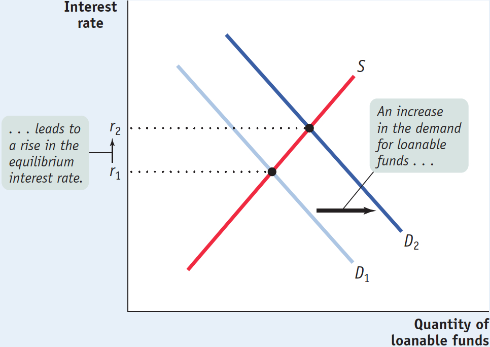
Figure 10-5 shows the effects of an increase in the demand for loanable funds. S is the supply of loanable funds, and D1 is the initial demand curve. The initial equilibrium interest rate is r1. An increase in the demand for loanable funds means that the quantity of funds demanded rises at any given interest rate, so the demand curve shifts rightward to D2. As a result, the equilibrium interest rate rises to r2.
10-5
An Increase in the Demand for Loanable Funds
The fact that an increase in the demand for loanable funds leads, other things equal, to a rise in the interest rate has one especially important implication: it tells us that increasing or persistent government budget deficits are cause for concern because an increase in the government’s deficit shifts the demand curve for loanable funds to the right, which leads to a higher interest rate. If the interest rate rises, businesses will cut back on their investment spending.
Crowding out occurs when a government budget deficit drives up the interest rate and leads to reduced investment spending.
So, other things equal, a rise in the government budget deficit tends to reduce overall investment spending. Economists call the negative effect of government budget deficits on investment spending crowding out. Concerns about crowding out are one key reason to worry about increasing or persistent budget deficits.
However, it’s important to add a qualification here: crowding out may not occur if the economy is depressed. When the economy is operating far below full employment, government spending can lead to higher incomes, and these higher incomes lead to increased savings at any given interest rate. Higher savings allows the government to borrow without raising interest rates. Many economists believe, for example, that the large budget deficits that the U.S. government ran from 2008 to 2013 in the face of a depressed economy caused little if any crowding out.
Shifts of the Supply of Loanable Funds Like the demand for loanable funds, the supply of loanable funds can shift. Among the factors that can cause the supply of loanable funds to shift are the following:
Changes in private savings behavior. A number of factors can cause the level of private savings to change at any given interest rate. For example, between 2000 and 2006 rising home prices in the United States made many homeowners feel richer, making them willing to spend more and save less. This had the effect of shifting the supply curve of loanable funds to the left.
Changes in net capital inflows. Capital flows into and out of a country can change as investors’ perceptions of that country change. For example, Greece experienced large net capital inflows after the creation of the euro, Europe’s common currency, in 1999, because investors believed that Greece’s adoption of the euro as its currency had made it a safe place to put their funds. By 2009, however, worries about the Greek government’s solvency (and the discovery that it had been understating its debt) led to a collapse in investor confidence, and the net inflow of funds dried up. The effect of shrinking capital inflows was to shift the supply curve in the Greek loanable funds market to the left.
In the mid-
2000s, the United States received large net capital inflows, with much of the money coming from China and the Middle East. Those inflows helped fuel a big increase in residential investment spending— newly constructed homes— from 2003 to 2006. As a result of the bursting of the U.S. housing bubble in 2006– 2007 and the subsequent deep recession, those inflows began to trail off in 2008.
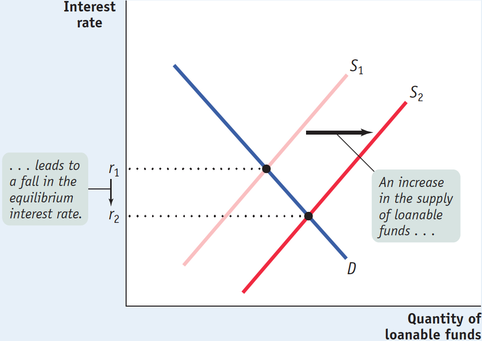
Figure 10-6 shows the effects of an increase in the supply of loanable funds. D is the demand for loanable funds, and S1 is the initial supply curve. The initial equilibrium interest rate is r1. An increase in the supply of loanable funds means that the quantity of funds supplied rises at any given interest rate, so the supply curve shifts rightward to S2. As a result, the equilibrium interest rate falls to r2.
10-6
An Increase in the Supply of Loanable Funds
Inflation and Interest Rates Anything that shifts either the supply of loanable funds curve or the demand for loanable funds curve changes the interest rate. Historically, major changes in interest rates have been driven by many factors, including changes in government policy and technological innovations that created new investment opportunities.
However, arguably the most important factor affecting interest rates over time—
To understand the effect of expected future inflation on interest rates, recall our discussion in Chapter 8 of the way inflation creates winners and losers—
Real interest rate = Nominal interest rate − Inflation rate
The true cost of borrowing is the real interest rate, not the nominal interest rate. To see why, suppose a firm borrows $10,000 for one year at a 10% nominal interest rate. At the end of the year, it must repay $11,000—
Similarly, the true payoff to lending is the real interest rate, not the nominal interest rate. Suppose that a bank makes a $10,000 loan for one year at a 10% nominal interest rate. At the end of the year, the bank receives an $11,000 repayment. But if the average level of prices rises by 10% per year, the purchasing power of the money the bank gets back is no more than that of the money it lent out. In real terms, the bank has made a zero-
Now we can add an important detail to our analysis of the loanable funds market. Figures 10-5 and 10-6 are drawn with the vertical axis measuring the nominal interest rate for a given expected future inflation rate. Why do we use the nominal interest rate rather than the real interest rate? Because in the real world neither borrowers nor lenders know what the future inflation rate will be when they make a deal. Actual loan contracts therefore specify a nominal interest rate rather than a real interest rate. Because we are holding the expected future inflation rate fixed in Figures 10-5 and 10-6, however, changes in the nominal interest rate also lead to changes in the real interest rate.
The expectations of borrowers and lenders about future inflation rates are normally based on recent experience. In the late 1970s, after a decade of high inflation, borrowers and lenders expected future inflation to be high. By the late 1990s, after a decade of fairly low inflation, borrowers and lenders expected future inflation to be low. And these changing expectations about future inflation had a strong effect on the nominal interest rate, largely explaining why nominal interest rates were much lower in the early years of the twenty-
Let’s look at how changes in the expected future rate of inflation are reflected in the loanable funds model.
In Figure 10-7, the curves S0 and D0 show the supply and demand for loanable funds given that the expected future rate of inflation is 0%. In that case, equilibrium is at E0, and the equilibrium nominal interest rate is 4%. Because expected future inflation is 0%, the equilibrium expected real interest rate over the life of the loan is also 4%.
10-7
The Fisher Effect
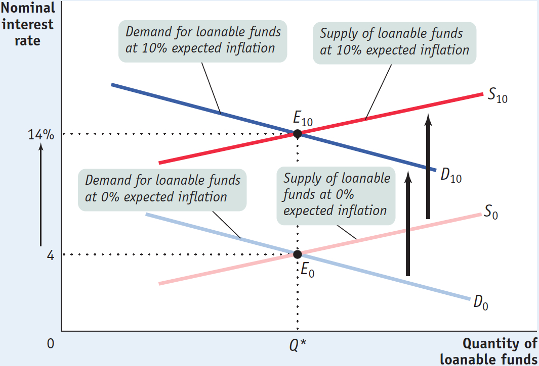
Now suppose that the expected future inflation rate rises to 10%. The demand curve for loanable funds shifts upward to D10: borrowers are now willing to borrow as much at a nominal interest rate of 14% as they were previously willing to borrow at 4%. That’s because with a 10% inflation rate, a 14% nominal interest rate corresponds to a 4% real interest rate. Similarly, the supply curve of loanable funds shifts upward to S10: lenders require a nominal interest rate of 14% to persuade them to lend as much as they would previously have lent at 4%. The new equilibrium is at E10: the result of an expected future inflation rate of 10% is that the equilibrium nominal interest rate rises from 4% to 14%.
According to the Fisher effect, an increase in expected future inflation drives up the nominal interest rate, leaving the expected real interest rate unchanged.
This situation can be summarized as a general principle, known as the Fisher effect (after the American economist Irving Fisher, who proposed it in 1930): the expected real interest rate is unaffected by changes in expected future inflation. According to the Fisher effect, an increase in expected future inflation drives up the nominal interest rate, where each additional percentage point of expected future inflation drives up the nominal interest rate by 1 percentage point. The central point is that both lenders and borrowers base their decisions on the expected real interest rate. As a result, a change in the expected rate of inflation does not affect the equilibrium quantity of loanable funds or the expected real interest rate; all it affects is the equilibrium nominal interest rate.
ECONOMICS in Action: Sixty Years of U.S. Interest Rates
Sixty Years of U.S. Interest Rates
There have been some large movements in U.S. interest rates dating back to the 1950s. These movements clearly show how both changes in expected future inflation and changes in the expected return on investment spending move interest rates.
Panel (a) of Figure 10-8 illustrates the first effect. It shows the average interest rate on bonds issued by the U.S. government—
10-8
Changes in U.S. Interest Rates Over Time
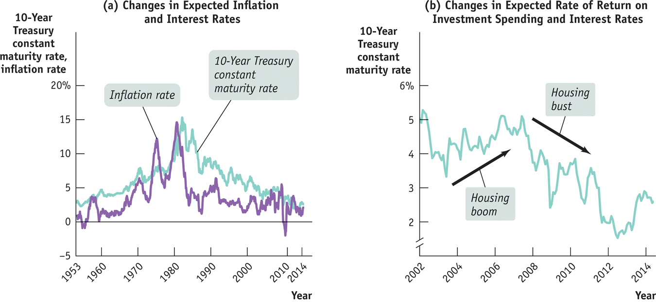
Panel (b) illustrates the second effect: changes in the expected return on investment spending and interest rates, with a “close-
Throughout this whole process, total savings was equal to total investment spending, and the rise and fall of the interest rate played a key role in matching lenders with borrowers.
Quick Review
The savings–
investment spending identity is an accounting fact: savings is equal to investment spending for the economy as a whole.The government is a source of savings when it runs a positive budget balance, a budget surplus. It is a source of dissavings when it runs a negative budget balance, a budget deficit.
Savings is equal to national savings plus net capital inflow, which may be either positive or negative.
When costs or benefits arrive at different times, you must take the complication created by time into account. This is done by transforming any dollars realized in the future into their present value.
The loanable funds market matches savers to borrowers. In equilibrium, only investment spending projects with an expected return greater than or equal to the equilibrium interest rate are funded.
Because the government competes with private borrowers in the loanable funds market, a government deficit can cause crowding out. However, crowding out is unlikely when the economy is in a slump.
Higher expected future inflation raises the nominal interest rate through the Fisher effect, leaving the real interest rate unchanged.
10-1
Question 10.1
Use a diagram of the loanable funds market to illustrate the effect of the following events on the equilibrium interest rate and investment spending.
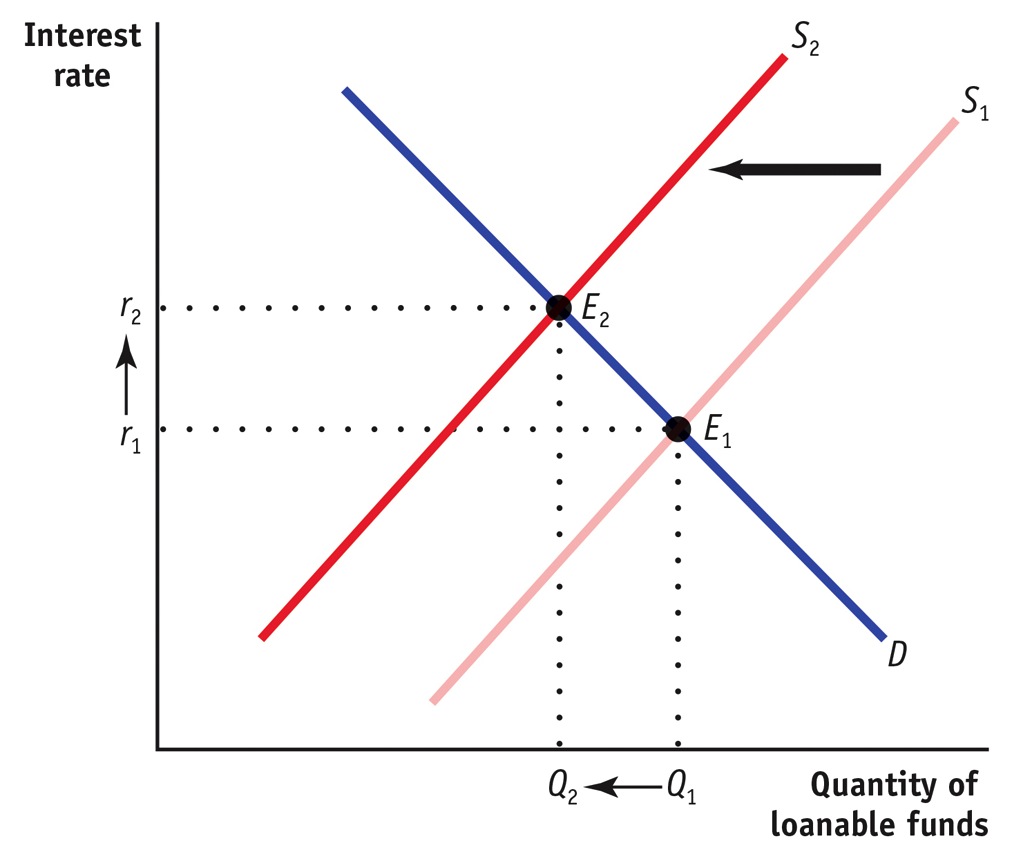
An economy is opened to international movements of capital, and a net capital inflow occurs.
As there is a net capital inflow into the economy, the supply of loanable funds increases. This is illustrated by the shift of the supply curve from S1 to S2 in the accompanying diagram. As the equilibrium moves from E1 to E2, the equilibrium interest rate falls from r1 to r2, and the equilibrium quantity of loanable funds increases from Q1 to Q2.

Retired people generally save less than working people at any interest rate. The proportion of retired people in the population goes up.
Savings fall due to the higher proportion of retired people, and the supply of loanable funds decreases. This is illustrated by the leftward shift of the supply curve from S1 to S2 in the accompanying diagram. The equilibrium moves from E1 to E2, the equilibrium interest rate rises from r1 to r2, and the equilibrium quantity of loanable funds falls from Q1 to Q2.
Question 10.2
Explain what is wrong with the following statement: “Savings and investment spending may not be equal in the economy as a whole because when the interest rate rises, households will want to save more money than businesses will want to invest.”
We know from the loanable funds market that as the interest rate rises, households want to save more and consume less. But at the same time, an increase in the interest rate lowers the number of investment spending projects with returns at least as high as the interest rate. The statement “households will want to save more money than businesses will want to invest” cannot represent an equilibrium in the loanable funds market because it says that the quantity of loanable funds offered exceeds the quantity of loanable funds demanded. If that were to occur, the interest rate must fall to make the quantity of loanable funds offered equal to the quantity of loanable funds demanded.
Question 10.3
Suppose that expected inflation rises from 3% to 6%.
How will the real interest rate be affected by this change?
The real interest rate will not change. According to the Fisher effect, an increase in expected inflation drives up the nominal interest rate, leaving the real interest rate unchanged.
How will the nominal interest rate be affected by this change?
The nominal interest rate will rise by 3%. Each additional percentage point of expected inflation drives up the nominal interest rate by 1 percentage point.
What will happen to the equilibrium quantity of loanable funds?
As we saw in Figure 10-7, as long as inflation is expected, it does not affect the equilibrium quantity of loanable funds. Both the supply and demand curves for loanable funds are pushed upward, leaving the equilibrium quantity of loanable funds unchanged.
Solutions appear at back of book.