Money, Output, and Prices in the Long Run
Through its expansionary and contractionary effects, monetary policy is generally the policy tool of choice to help stabilize the economy. However, not all actions by central banks are productive. In particular, central banks sometimes print money not to fight a recessionary gap but to help the government pay its bills, an action that typically destabilizes the economy.
What happens when a change in the money supply pushes the economy away from, rather than toward, long-
Short-Run and Long-Run Effects of an Increase in the Money Supply
To analyze the long-
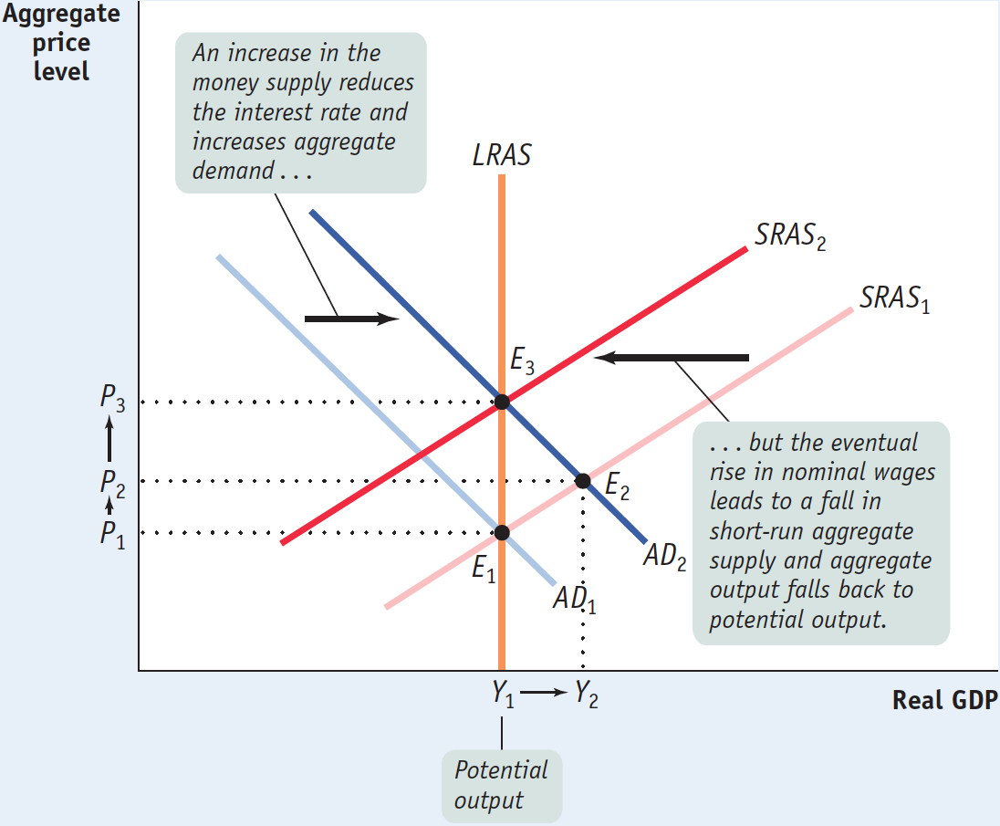
Figure 15-11 shows the short-
15-11
The Short-

Here, the economy begins at E1, a point of short-
The economy reaches a new short-
Now suppose there is an increase in the money supply. Other things equal, an increase in the money supply reduces the interest rate, which increases investment spending, which leads to a further rise in consumer spending, and so on. So an increase in the money supply increases the quantity of goods and services demanded, shifting the AD curve rightward, to AD2. In the short run, the economy moves to a new short-
But the aggregate output level, Y2, is above potential output. As a result, nominal wages will rise over time, causing the short-
We won’t describe the effects of a monetary contraction in detail, but the same logic applies. In the short run, a fall in the money supply leads to a fall in aggregate output as the economy moves down the short-
Monetary Neutrality
How much does a change in the money supply change the aggregate price level in the long run? The answer is that a change in the money supply leads to an equal proportional change in the aggregate price level in the long run. For example, if the money supply falls 25%, the aggregate price level falls 25% in the long run; if the money supply rises 50%, the aggregate price level rises 50% in the long run.
How do we know this? Consider the following thought experiment: suppose all prices in the economy—
We can state this argument in reverse: if the economy starts out in long-
According to the concept of monetary neutrality, changes in the money supply have no real effects on the economy.
This analysis demonstrates the concept known as monetary neutrality, in which changes in the money supply have no real effects on the economy. In the long run, the only effect of an increase in the money supply is to raise the aggregate price level by an equal percentage. Economists argue that money is neutral in the long run.
This is, however, a good time to recall the dictum of John Maynard Keynes: “In the long run we are all dead.” In the long run, changes in the money supply don’t have any effect on real GDP, interest rates, or anything else except the price level. But it would be foolish to conclude from this that the Fed is irrelevant. Monetary policy does have powerful real effects on the economy in the short run, often making the difference between recession and expansion. And that matters a lot for society’s welfare.
Changes in the Money Supply and the Interest Rate in the Long Run
In the short run, an increase in the money supply leads to a fall in the interest rate, and a decrease in the money supply leads to a rise in the interest rate. In the long run, however, changes in the money supply don’t affect the interest rate.
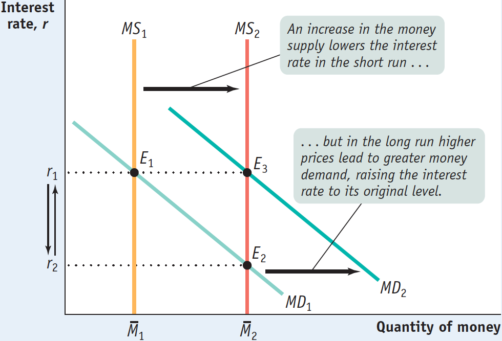
Figure 15-12 shows why. It shows the money supply curve and the money demand curve before and after the Fed increases the money supply. We assume that the economy is initially at E1, in long- . The initial equilibrium interest rate, determined by the intersection of the money demand curve MD1 and the money supply curve MS1, is r1.
15-12
The Long-

 to
to  pushes the interest rate down from r1 to r2 and the economy moves to E2, a short-
Now suppose the money supply increases from  to
to  . In the short run, the economy moves from E1 to E2 and the interest rate falls from r1 to r2. Over time, however, the aggregate price level rises, and this raises money demand, shifting the money demand curve rightward from MD1 to MD2. The economy moves to a new long-
And it turns out that the long-
So a 50% increase in the money supply raises the aggregate price level by 50%, which increases the quantity of money demanded at any given interest rate by 50%. As a result, the quantity of money demanded at the initial interest rate, r1, rises exactly as much as the money supply—
!worldview! ECONOMICS in Action: International Evidence of Monetary Neutrality
International Evidence of Monetary Neutrality
These days monetary policy is quite similar among wealthy countries. Each major nation (or, in the case of the euro, the euro area) has a central bank that is insulated from political pressure. All of these central banks try to keep the aggregate price level roughly stable, which usually means inflation of at most 2% to 3% per year.
15-13
The Long-

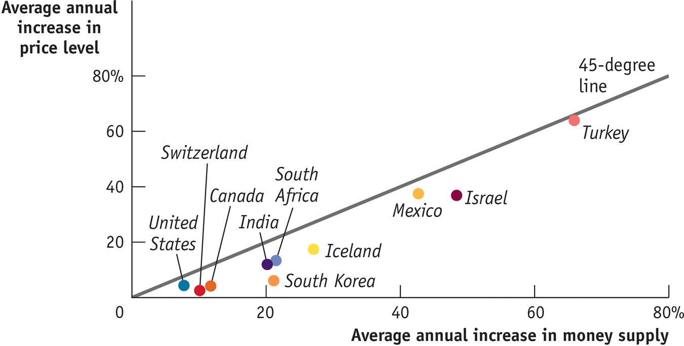
But if we look at a longer period and a wider group of countries, we see large differences in the growth of the money supply. Between 1970 and the present, the money supply rose only a few percent per year in some countries, such as Switzerland and the United States, but rose much more rapidly in some poorer countries, such as South Africa. These differences allow us to see whether it is really true that increases in the money supply lead, in the long run, to equal percent rises in the aggregate price level.
Figure 15-13 shows the annual percentage increases in the money supply and average annual increases in the aggregate price level—
In fact, the relationship isn’t exact, because other factors besides money affect the aggregate price level. But the scatter of points clearly lies close to a 45-
Quick Review
According to the concept of monetary neutrality, changes in the money supply do not affect real GDP, they only affect the aggregate price level. Economists believe that money is neutral in the long run.
In the long run, the equilibrium interest rate in the economy is unaffected by changes in the money supply.
15-4
Question 15.8
Assume the central bank increases the quantity of money by 25%, even though the economy is initially in both short-
run and long- run macroeconomic equilibrium. Describe the effects, in the short run and in the long run (giving numbers where possible), on the following. Aggregate output
Aggregate output rises in the short run, then falls back to equal potential output in the long run.
Aggregate price level
The aggregate price level rises in the short run, but by less than 25%. It rises further in the long run, for a total increase of 25%.
Interest rate
The interest rate falls in the short run, then rises back to its original level in the long run.
Question 15.9
Why does monetary policy affect the economy in the short run but not in the long run?
In the short run, a change in the interest rate alters the economy because it affects investment spending, which in turn affects aggregate demand and real GDP through the multiplier process. However, in the long run, changes in consumer spending and investment spending will eventually result in changes in nominal wages and the nominal prices of other factors of production. For example, an expansionary monetary policy will eventually cause a rise in factor prices; a contractionary policy will eventually cause a fall in factor prices. In response, the short-run aggregate supply curve will shift to move the economy back to longrun equilibrium. So in the long run monetary policy has no effect on the economy.
Solutions appear at back of book.
PIMCO Bets on Cheap Money
Pacific Investment Management Company, generally known as PIMCO, is one of the world’s largest investment companies. Among other things, it runs PIMCO Total Return, the world’s largest mutual fund. Bill Gross, who headed PIMCO from 1971 until 2014, was legendary for his ability to predict trends in financial markets, especially bond markets, where PIMCO does much of its investing.

In the fall of 2009, Gross decided to put more of PIMCO’s assets into long-
What lay behind PIMCO’s bet? Gross explained the firm’s thinking in his September 2009 commentary. He suggested that unemployment was likely to stay high and inflation low. “Global policy rates,” he asserted—
PIMCO’s view was in sharp contrast to those of other investors: Morgan Stanley expected long-
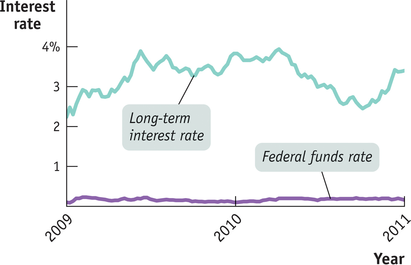
Who was right? PIMCO, mostly. As Figure 15-14 shows, the federal funds rate stayed near zero, and long-
15-14
The Federal Funds Rate and Long-

Bill Gross’s foresight, however, was a lot less accurate in 2011. Anticipating a significantly stronger U.S. economy by mid-
QUESTIONS FOR THOUGHT
Question 15.10
Why did PIMCO’s view that unemployment would stay high and inflation low lead to a forecast that policy interest rates would remain low for an extended period?
Why did PIMCO’s view that unemployment would stay high and inflation low lead to a forecast that policy interest rates would remain low for an extended period?Question 15.11
Why would low policy rates suggest low long-
term interest rates? Why would low policy rates suggest low long-term interest rates? Question 15.12
What might have caused long-
term interest rates to rise in late 2010, even though the federal funds rate was still zero? What might have caused long-term interest rates to rise in late 2010, even though the federal funds rate was still zero?