Budgets and Optimal Consumption
The principle of diminishing marginal utility explains why most people eventually reach a limit, even at an all-
What do we mean by cost? As always, the fundamental measure of cost is opportunity cost. Because the amount of money a consumer can spend is limited, a decision to consume more of one good is also a decision to consume less of some other good.
Budget Constraints and Budget Lines
Consider Sammy, whose appetite is exclusively for clams and potatoes (there’s no accounting for tastes). He has a weekly income of $20 and since, given his appetite, more of either good is better than less, he spends all of it on clams and potatoes. We will assume that clams cost $4 per pound and potatoes cost $2 per pound. What are his possible choices?
Whatever Sammy chooses, we know that the cost of his consumption bundle cannot exceed his income, the amount of money he has to spend. That is,

A budget constraint requires that the cost of a consumer’s consumption bundle be no more than the consumer’s income.
A consumer’s consumption possibilities is the set of all consumption bundles that can be consumed given the consumer’s income and prevailing prices.
Consumers always have limited income, which constrains how much they can consume. So the requirement illustrated by Equation 10-
Figure 10-2 shows Sammy’s consumption possibilities. The quantity of clams in his consumption bundle is measured on the horizontal axis and the quantity of potatoes on the vertical axis. The downward-
10-2
The Budget Line
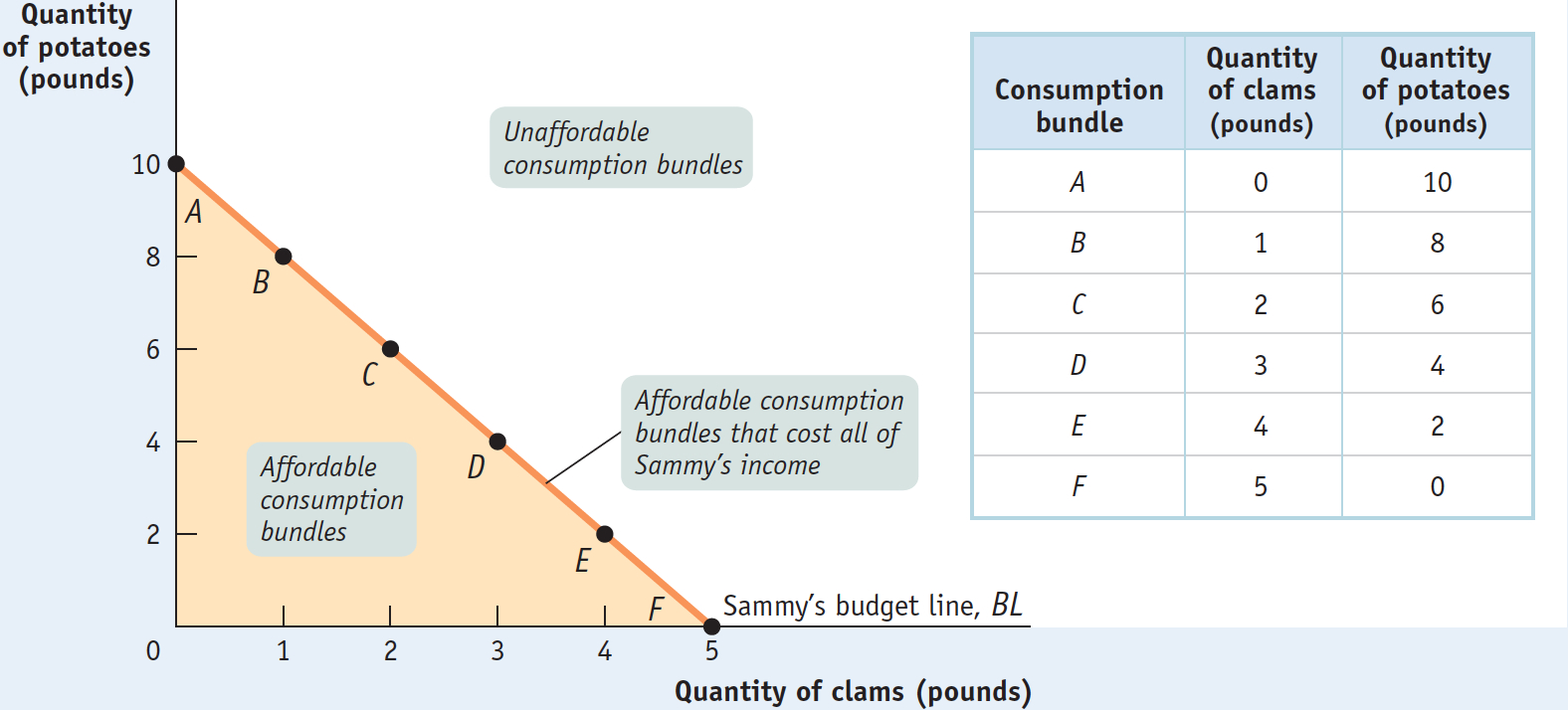
As an example of one of the points, let’s look at point C, representing 2 pounds of clams and 6 pounds of potatoes, and check whether it satisfies Sammy’s budget constraint. The cost of bundle C is 6 pounds of potatoes × $2 per pound + 2 pounds of clams × $4 per pound = $12 + $8 = $20. So bundle C does indeed satisfy Sammy’s budget constraint: it costs no more than his weekly income of $20. In fact, bundle C costs exactly as much as Sammy’s income. By doing the arithmetic, you can check that all the other points lying on the downward-
A consumer’s budget line shows the consumption bundles available to a consumer who spends all of his or her income.
The downward-
Do we need to consider the other bundles in Sammy’s consumption possibilities, the ones that lie within the shaded region in Figure 10-2 bounded by the budget line? The answer is, for all practical situations, no: as long as Sammy continues to get positive marginal utility from consuming either good (in other words, Sammy doesn’t get satiated)—and he doesn’t get any utility from saving income rather than spending it, then he will always choose to consume a bundle that lies on his budget line and not within the shaded area.
Given his $20 per week budget, which point on his budget line will Sammy choose?
Optimal Consumption Choice
A consumer’s optimal consumption bundle is the consumption bundle that maximizes the consumer’s total utility given his or her budget constraint.
Because Sammy has a budget constraint, which means that he will consume a consumption bundle on the budget line, a choice to consume a given quantity of clams also determines his potato consumption, and vice versa. We want to find the consumption bundle—
Table 10-1 shows how much utility Sammy gets from different levels of consumption of clams and potatoes, respectively. According to the table, Sammy has a healthy appetite; the more of either good he consumes, the higher his utility.
10-1
Sammy’s Utility from Clam and Potato Consumption
|
Utility from clam consumption |
Utility from potato consumption |
||
|---|---|---|---|
|
Quantity of clams (pounds) |
Utility from clams (utils) |
Quantity of potatoes (pounds) |
Utility from potatoes (utils) |
|
0 |
0 |
0 |
0 |
|
1 |
15 |
1 |
11.5 |
|
2 |
25 |
2 |
21.4 |
|
3 |
31 |
3 |
29.8 |
|
4 |
34 |
4 |
36.8 |
|
5 |
36 |
5 |
42.5 |
|
6 |
47.0 |
||
|
7 |
50.5 |
||
|
8 |
53.2 |
||
|
9 |
55.2 |
||
|
10 |
56.7 |
||
TABLE 10-
But because he has a limited budget, he must make a trade-
Table 10-2 shows how his total utility varies for the different consumption bundles along his budget line. Each of six possible consumption bundles, A through F from Figure 10-2, is given in the first column. The second column shows the level of clam consumption corresponding to each choice. The third column shows the utility Sammy gets from consuming those clams. The fourth column shows the quantity of potatoes Sammy can afford given the level of clam consumption; this quantity goes down as his clam consumption goes up, because he is sliding down the budget line. The fifth column shows the utility he gets from consuming those potatoes. And the final column shows his total utility. In this example, Sammy’s total utility is the sum of the utility he gets from clams and the utility he gets from potatoes.
10-2
Sammy’s Budget and Total Utility
|
Consumption bundle |
Quantity of clams (pounds) |
Utility from clams (utils) |
Quantity of potatoes (pounds) |
Utility from potatoes (utils) |
Total utility (utils) |
|---|---|---|---|---|---|
|
A |
0 |
0 |
10 |
56.7 |
56.7 |
|
B |
1 |
15 |
8 |
53.2 |
68.2 |
|
C |
2 |
25 |
6 |
47.0 |
72.0 |
|
D |
3 |
31 |
4 |
36.8 |
67.8 |
|
E |
4 |
34 |
2 |
21.4 |
55.4 |
|
F |
5 |
36 |
0 |
0 |
36.0 |
TABLE 10-
Figure 10-3 gives a visual representation of the data shown in Table 10-2. Panel (a) shows Sammy’s budget line, to remind us that when he decides to consume more clams he is also deciding to consume fewer potatoes. Panel (b) then shows how his total utility depends on that choice. The horizontal axis in panel (b) has two sets of labels: it shows both the quantity of clams, increasing from left to right, and the quantity of potatoes, increasing from right to left.
10-3
Optimal Consumption Bundle
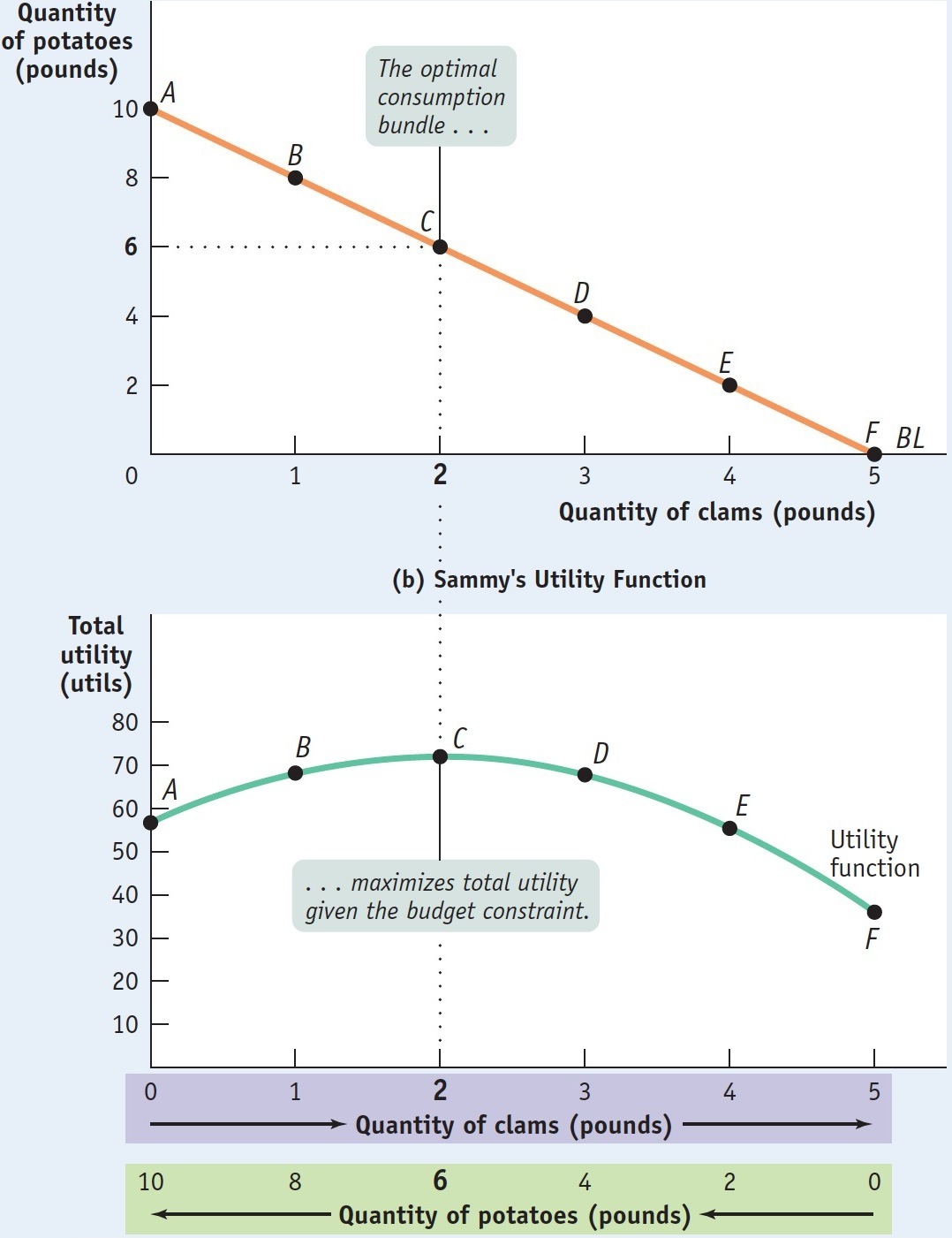
The reason we can use the same axis to represent consumption of both goods is, of course, the budget line: the more pounds of clams Sammy consumes, the fewer pounds of potatoes he can afford, and vice versa.
Clearly, the consumption bundle that makes the best of the trade-
As always, we can find the highest point of the curve by direct observation. We can see from Figure 10-3 that Sammy’s total utility is maximized at point C—that his optimal consumption bundle contains 2 pounds of clams and 6 pounds of potatoes. But we know that we usually gain more insight into “how much” problems when we use marginal analysis. So in the next section we turn to representing and solving the optimal consumption choice problem with marginal analysis.
Food for Thought on Budget Constraints
Budget constraints aren’t just about money. In fact, there are many other budget constraints affecting our lives. You face a budget constraint if you have a limited amount of closet space for your clothes. All of us face a budget constraint on time: there are only so many hours in the day.
And people trying to lose weight on the Weight Watchers plan face a budget constraint on the foods they eat.
The Weight Watchers plan assigns each food a certain number of points. A 4-
In other words, a dieter on the Weight Watchers plan is just like a consumer choosing a consumption bundle: points are the equivalent of prices, and the overall point limit is the equivalent of total income.
ECONOMICS in Action: The Great Condiment Craze
The Great Condiment Craze
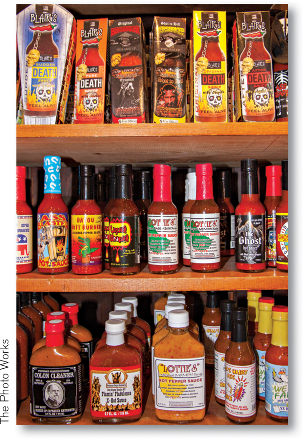
Those of us of a certain age remember when the only kind of mustard available in American grocery stores was a runny, fluorescent yellow concoction packaged in plastic squeeze bottles. Ditto for ketchup and mayonnaise—
No longer. Americans have developed an intense liking for condiments—
So what happened? Tastes changed and budgets changed. Spurred by the severe recession that began in 2007, more budget-
The explosion of varieties stems from the fact that it’s fairly easy to make bottled condiments. This enables smaller companies to experiment with exotic flavors, finding the ones that appeal to consumers’ increasingly sophisticated tastes. Eventually, the flavors that attract a significant following are picked up by the larger companies such as Kraft. As one industry analyst put it, “People want cheaper, more specialized gourmet products. It’s like fashion.”
As the economy has slowly recovered in recent years, restaurant dining has picked up. However, American home cooking appears to have been forever changed by the great condiment craze. Consumers continue to purchase a wide variety of premium condiments to add zest to their home-
Quick Review
The budget constraint requires that a consumer’s total expenditure be no more than his or her income. The set of consumption bundles that satisfy the budget constraint is the consumer’s consumption possibilities.
A consumer who spends all of his or her income chooses a point on his or her budget line. The budget line slopes downward because on the budget line a consumer must consume less of one good in order to consume more of another.
The consumption choice that maximizes total utility given the consumer’s budget constraint is the optimal consumption bundle. It must lie on the consumer’s budget line.
10-2
Question 10.4
In the following two examples, find all the consumption bundles that lie on the consumer’s budget line. Illustrate these consumption possibilities in a diagram and draw the budget line through them.
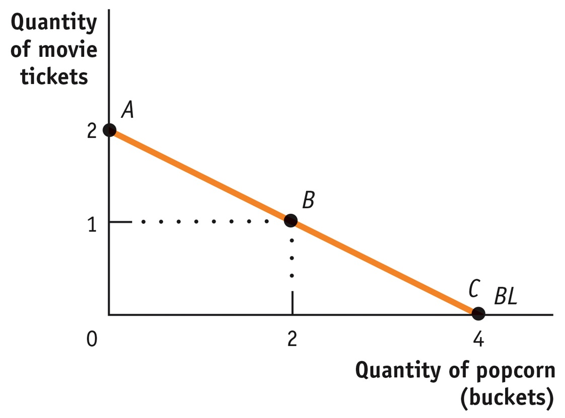
The consumption bundle consists of movie tickets and buckets of popcorn. The price of each ticket is $10.00, the price of each bucket of popcorn is $5.00, and the consumer’s income is $20.00. In your diagram, put movie tickets on the vertical axis and buckets of popcorn on the horizontal axis.
The accompanying table shows the consumer’s consumption possibilities, A through C. These consumption possibilities are plotted in the accompanying diagram, along with the consumer’s budget line, BL.Consumption bundle
Quantity of popcorn (buckets)
Quantity of movie tickets
A
0
2
B
2
1
C
4
0
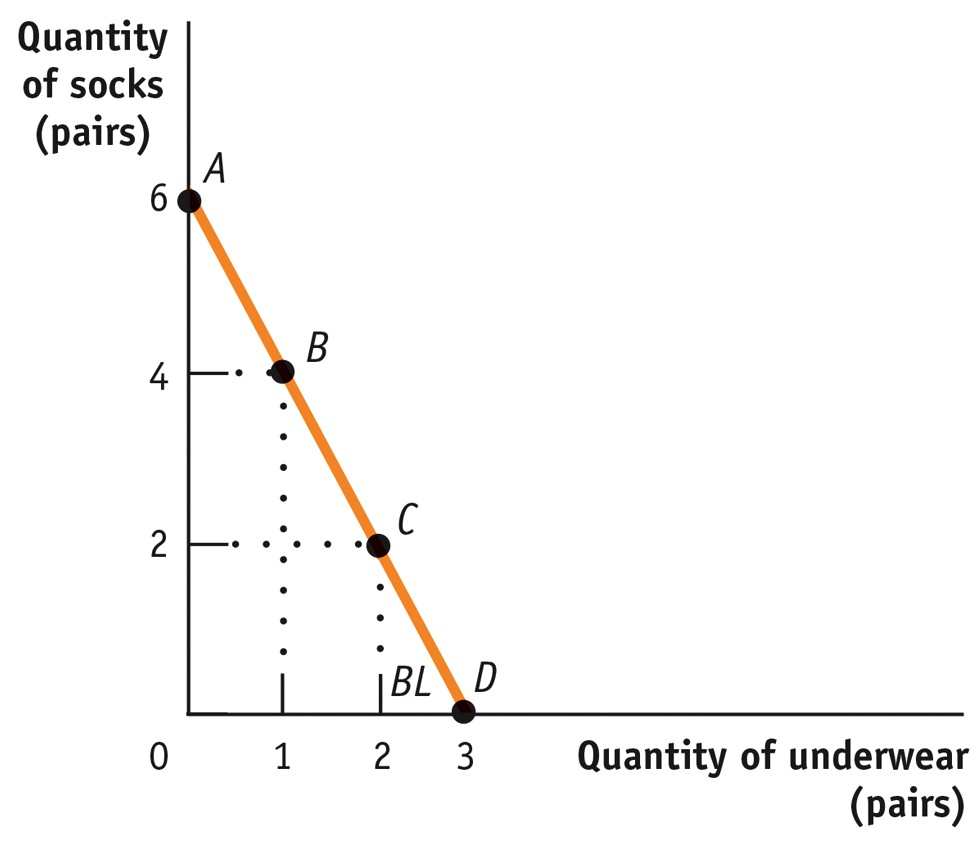
The consumption bundle consists of underwear and socks. The price of each pair of underwear is $4.00, the price of each pair of socks is $2.00, and the consumer’s income is $12.00. In your diagram, put pairs of socks on the vertical axis and pairs of underwear on the horizontal axis.
The accompanying table shows the consumer’s consumption possibilities, A through D. These consumption possibilities are plotted in the accompanying diagram, along with the consumer’s budget line, BL.Consumption bundle
Quantity of underwear (pairs)
Quantity of socks (pairs)
A
0
6
B
1
4
C
2
2
D
3
0
Solutions appear at back of book.