Let’s return now to Ingrid’s consumption choices. In the situation we’ve considered, her income was $2,400 per month, housing cost $150 per room, and restaurant meals cost $30 each. Her optimal consumption bundle, as seen in Figure 10A-7, contained 8 rooms and 40 restaurant meals.

Let’s now ask how her consumption choice would change if either the rent per room or her income changed. As we’ll see, we can put these pieces together to deepen our understanding of consumer demand.

Suppose that for some reason there is a sharp increase in housing prices. Ingrid must now pay $600 per room instead of $150. Meanwhile, the price of restaurant meals and her income remain unchanged. How does this change affect her consumption choices?

When the price of rooms rises, the relative price of rooms in terms of restaurant meals rises; as a result, Ingrid’s budget line changes (for the worse—but we’ll get to that). She responds to that change by choosing a new consumption bundle.

Figure 10A-12 shows Ingrid’s original (BL₁) and new (BL₂) budget lines—again, under the assumption that her income remains constant at $2,400 per month. With housing costing $150 per room and a restaurant meal costing $30, her budget line, BL₁, intersected the horizontal axis at 16 rooms and the vertical axis at 80 restaurant meals. After the price of a room rises to $600 per room, the budget line, BL₂, still hits the vertical axis at 80 restaurant meals, but it hits the horizontal axis at only 4 rooms. That’s because we know from Equation (10A-9) that the new horizontal intercept of the budget line is now $2,400/$600 = 4. Her budget line has rotated inward and become steeper, reflecting the new, higher relative price of a room in terms of restaurant meals.

10A-12

Effects of a Price Increase on the Budget Line

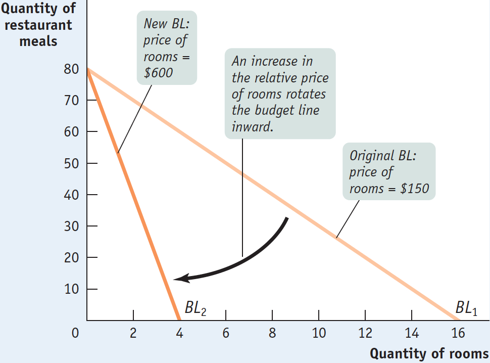
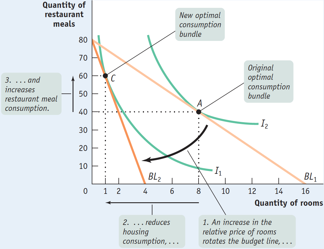
Figure 10A-13 shows how Ingrid responds to her new circumstances. Her original optimal consumption bundle consists of 8 rooms and 40 meals. After her budget line rotates in response to the change in relative price, she finds her new optimal consumption bundle by choosing the point on BL₂ that brings her to as high an indifference curve as possible. At the new optimal consumption bundle, she consumes fewer rooms and more restaurant meals than before: 1 room and 60 restaurant meals.

10A-13

Responding to a Price Increase

Why does Ingrid’s consumption of rooms fall? Part—but only part—of the reason is that the rise in the price of rooms reduces her purchasing power, making her poorer. That is, the higher relative price of rooms rotates her budget line inward toward the origin, reducing her consumption possibilities and putting her on a lower indifference curve. In a sense, when she faces a higher price of housing, it’s as if her income declined.

To understand this effect, and to see why it isn’t the whole story, let’s consider a different change in Ingrid’s circumstances: a change in her income.

In Chapter 3 we learned about the individual demand curve, which shows how a consumer’s consumption choice will change as the price of one good changes, holding income and the prices of other goods constant. That is, movement along the individual demand curve primarily shows the substitution effect, as we learned in Chapter 10—how quantity consumed changes in response to changes in the relative price of the two goods. But we can also ask how the consumption choice will change if income changes, holding relative price constant.

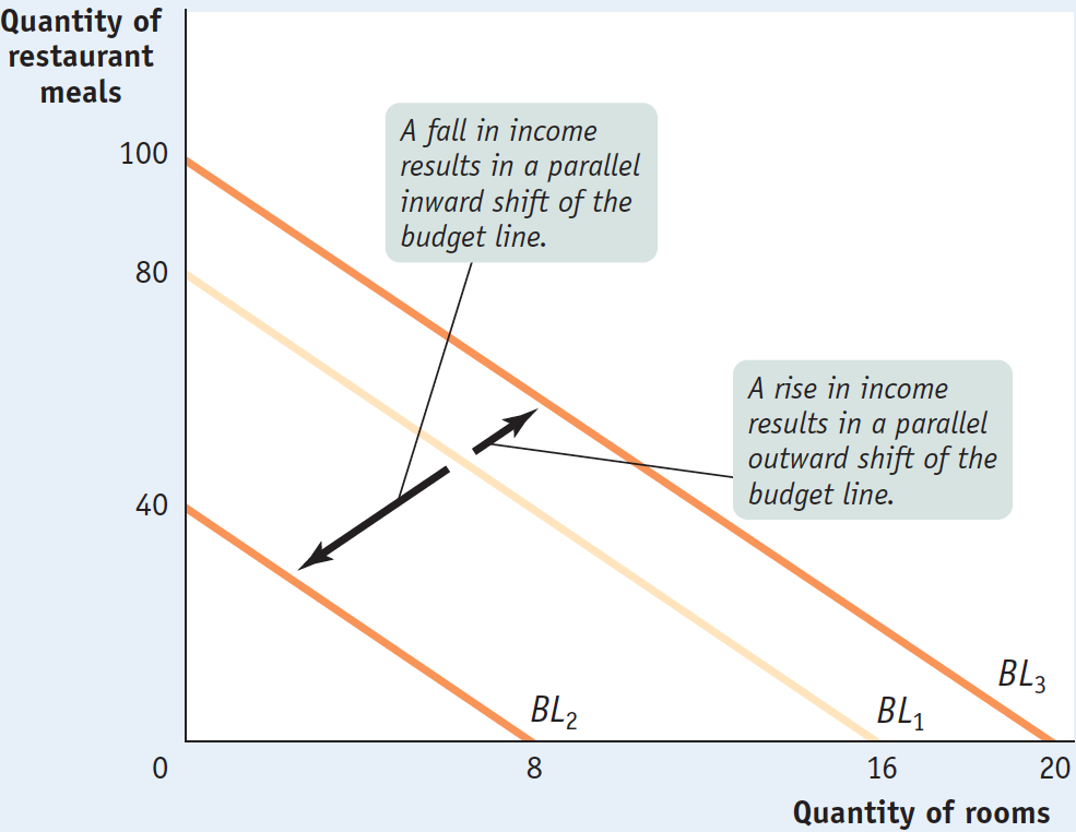
Before we proceed, it’s important to understand how a change in income, holding relative price constant, affects the budget line. Suppose that Ingrid’s income fell from $2,400 to $1,200 and we hold prices constant at $150 per room and $30 per restaurant meal. As a result, the maximum number of rooms she can afford drops from 16 to 8, and the maximum number of restaurant meals drops from 80 to 40. In other words, Ingrid’s consumption possibilities have shrunk, as shown by the parallel inward shift of the budget line in Figure 10A-14 from BL₁ to BL₂. It’s a parallel shift because the slope of the budget line—the relative price—remains unchanged when income changes. Alternatively, suppose Ingrid’s income rises from $2,400 to $3,000. She can now afford a maximum of 20 rooms or 100 meals, leading to a parallel outward shift of the budget line—the shift from BL₁ to BL₃ in Figure 10A-14. In this case, Ingrid’s consumption possibilities have expanded.

10A-14

Effect of a Change in Income on the Budget Line

Now we are ready to consider how Ingrid responds to a direct change in income—that is, a change in her income level holding relative price constant. Figure 10A-15 compares Ingrid’s budget line and optimal consumption choice at an income of $2,400 per month (BL₁) with her budget line and optimal consumption choice at an income of $1,200 per month (BL₂), keeping prices constant at $150 per room and $30 per restaurant meal. Point A is Ingrid’s optimal consumption bundle at an income of $2,400, and point B is her optimal consumption bundle at an income of $1,200. In each case, her optimal consumption bundle is given by the point at which the budget line is tangent to the indifference curve. As you can see, at the lower income her budget line shifts inward compared to her budget line at the higher income but maintains the same slope because relative price has not changed.

10A-15

Income and Consumption: Normal Goods

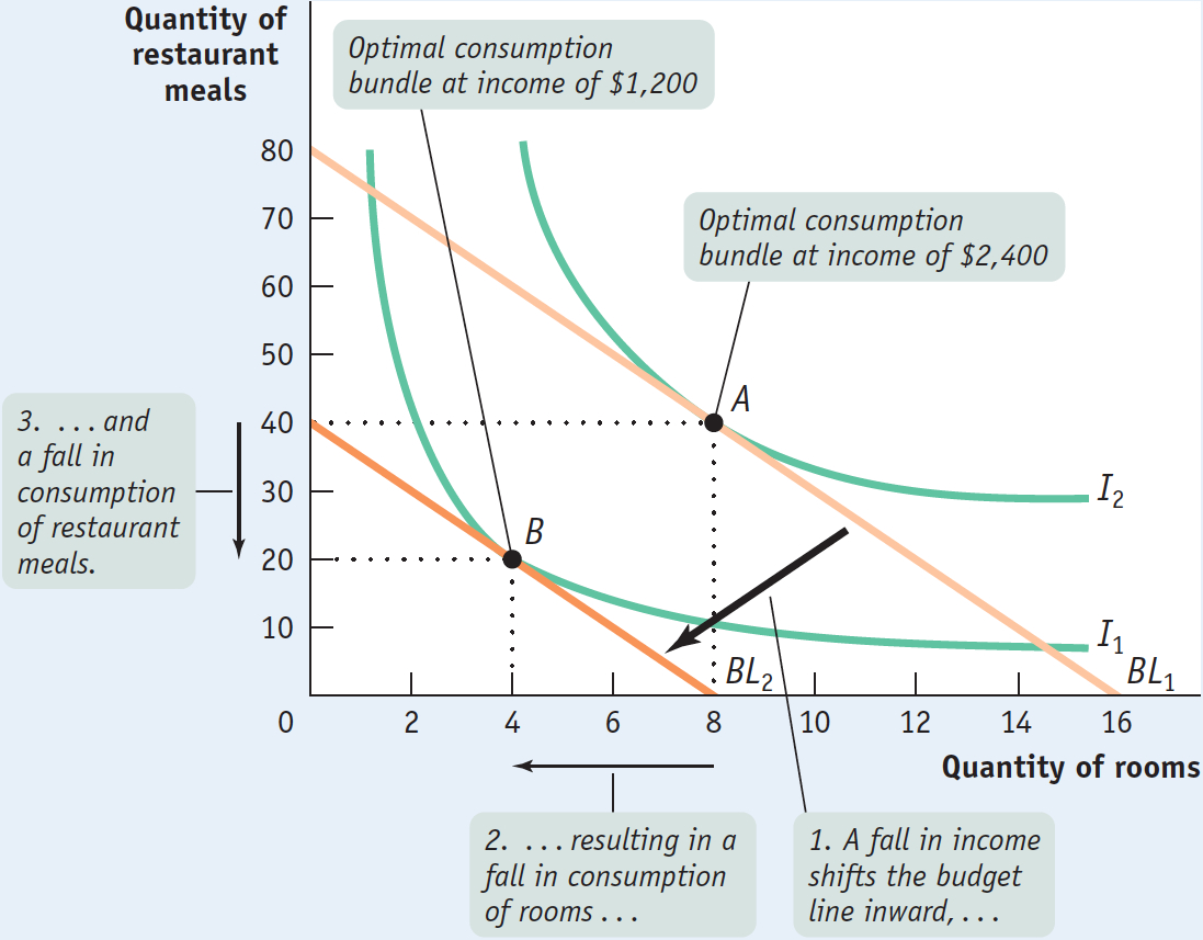
This means that she must reduce her consumption of either housing or restaurant meals, or both. As a result, she is at a lower level of total utility, represented by a lower indifference curve.

As it turns out, Ingrid chooses to consume less of both goods when her income falls: as her income goes from $2,400 to $1,200, her consumption of housing falls from 8 to 4 rooms and her consumption of restaurant meals falls from 40 to 20. This is because in her utility function both goods are normal goods, as defined in Chapter 3: goods for which demand increases when income rises and for which demand decreases when income falls.

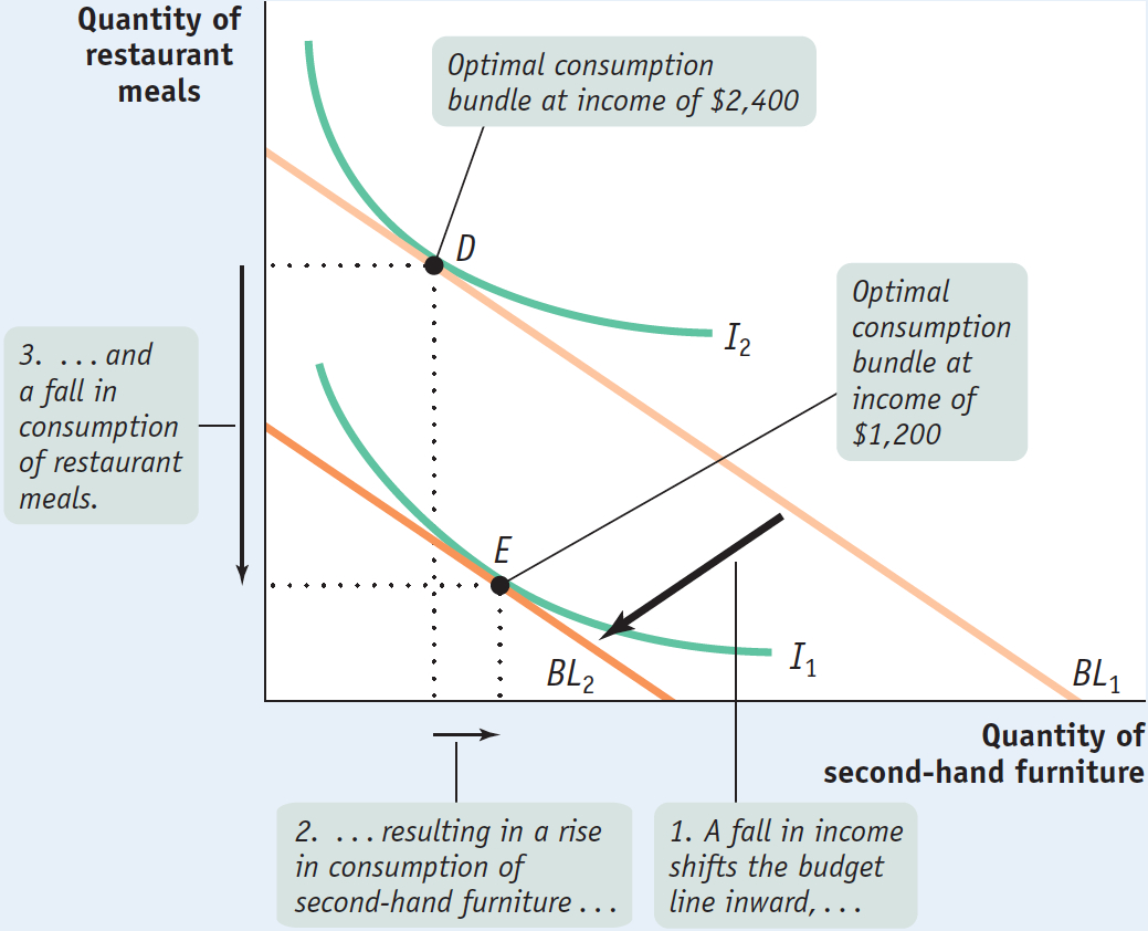
Although most goods are normal goods, we also pointed out in Chapter 3 that some goods are inferior goods, goods for which demand moves in the opposite direction to the change in income: demand decreases when income rises, and demand increases when income falls. An example might be second-hand furniture. Whether a good is an inferior good depends on the consumer’s indifference curve map. Figure 10A-16 illustrates such a case, where second−hand furniture is measured on the horizontal axis and restaurant meals are measured on the vertical axis. Note that when Ingrid’s income falls from $2,400 (BL₁) to $1,200 (BL₂), and her optimal consumption bundle goes from D to E, her consumption of second-hand furniture increases—implying that second-hand furniture is an inferior good. Simultaneously, her consumption of restaurant meals decreases—implying that restaurant meals are a normal good.

10A-16

Income and Consumption: An Inferior Good

Now that we have examined the effects of a change in income, we can return to the issue of a change in price—and show in a more specific way that the effect of a higher price on demand has an income component.

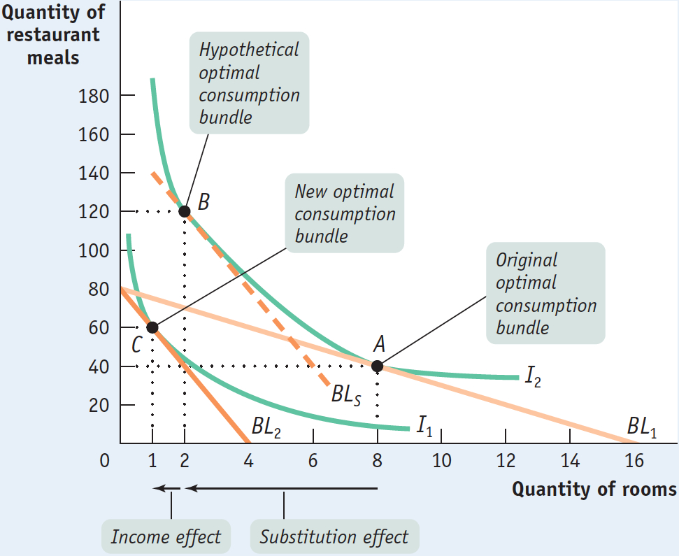
Figure 10A-17 shows, once again, Ingrid’s original (BL₁) and new (BL₂) budget lines and consumption choices with a monthly income of $2,400. At a housing price of $150 per room, Ingrid chooses the consumption bundle at A; at a housing price of $600 per room, she chooses the consumption bundle at C.

10A-17

Income and Substitution Effects

Let’s notice again what happens to Ingrid’s budget line after the increase in the price of housing. It continues to hit the vertical axis at 80 restaurant meals; that is, if Ingrid were to spend all her income on restaurant meals, the increase in the price of housing would not affect her. But the new budget line hits the horizontal axis at only 4 rooms. So the budget line has rotated, shifting inward and becoming steeper, as a consequence of the rise in the relative price of rooms.

We already know what happens: Ingrid’s consumption of housing falls from 8 rooms to 1 room. But the figure suggests that there are two reasons for the fall in Ingrid’s housing consumption. One reason she consumes fewer rooms is that, because of the higher relative price of rooms, the opportunity cost of a room measured in restaurant meals—the quantity of restaurant meals she must give up to consume an additional room—has increased. This change in opportunity cost, which is reflected in the steeper slope of the budget line, gives her an incentive to substitute restaurant meals in place of rooms in her consumption.

But the other reason Ingrid consumes fewer rooms after their price increases is that the rise in the price of rooms makes her poorer. True, her money income hasn’t changed. But she must pay more for rooms, and as a result her budget line has rotated inward. So she cannot reach the same level of total utility as before, meaning that her real income has fallen. That is why she ends up on a lower indifference curve.

In the real world, these effects—an increase in the price of a good raises its opportunity cost and also makes consumers poorer—usually go together. But in our imagination we can separate them. In Chapter 10 we introduced the distinction between the substitution effect of a price change (the change in consumption that arises from the substitution of the good that is now relatively cheaper in place of the good that is now relatively more expensive) and the income effect (the change in consumption caused by the change in purchasing power arising from a price change). Now we can show these two effects more clearly.

To isolate the substitution effect, let’s temporarily change the story about why Ingrid faces an increase in rent: it’s not that housing has become more expensive, it’s the fact that she has moved from Cincinnati to San Jose, where rents are higher. But let’s consider a hypothetical scenario—let’s suppose momentarily that she earns more in San Jose and that the higher income is just enough to compensate her for the higher price of housing, so that her total utility is exactly the same as before.

Figure 10A-17 shows her situation before and after the move. The bundle labeled A represents Ingrid’s original consumption choice: 8 rooms and 40 restaurant meals. When she moves to San Jose, she faces a higher price of housing, so her budget line becomes steeper. But we have just assumed that her move increases her income by just enough to compensate for the higher price of housing—that is, just enough to let her reach the original indifference curve. So her new hypothetical optimal consumption bundle is at B, where the steeper dashed hypothetical budget line (BL_S) is just tangent to the original indifference curve (I₂). By assuming that we have compensated Ingrid for the loss in purchasing power due to the increase in the price of housing, we isolate the pure substitution effect of the change in relative price on her consumption.

At B, Ingrid’s consumption bundle contains 2 rooms and 120 restaurant meals. This costs $4,800 (2 rooms at $600 each, and 120 meals at $30 each). So if Ingrid faces an increase in the price of housing from $150 to $600 per room, but also experiences a rise in her income from $2,400 to $4,800 per month, she ends up with the same level of total utility.

The movement from A to B is the pure substitution effect of the price change. It is the effect on Ingrid’s consumption choice when we change the relative price of housing while keeping her total utility constant.

Now that we have isolated the substitution effect, we can bring back the income effect of the price change. That’s easy: we just go back to the original story, in which Ingrid faces an increase in the price of housing without any rise in income. We already know that this leads her to C in Figure 10A-17. But we can think of the move from A to C as taking place in two steps. First, Ingrid moves from A to B, the substitution effect of the change in relative price. Then we take away the extra income needed to keep her on the original indifference curve, causing her to move to C. The movement from B to C is the additional change in Ingrid’s demand that results because the increase in housing prices actually reduces her utility. So this is the income effect of the price change.

We can use Figure 10A-17 to confirm that rooms are a normal good in Ingrid’s preferences. For normal goods, the income effect and the substitution effect work in the same direction: a price increase induces a fall in quantity consumed by the substitution effect (the move from A to B) and a fall in quantity consumed by the income effect (the move from B to C). That’s why demand curves for normal goods always slope downward.

What would have happened as a result of the increase in the price of housing if, instead of being a normal good, rooms had been an inferior good for Ingrid? First, the movement from A to B depicted in Figure 10A-17, the substitution effect, would remain unchanged. But an income change causes quantity consumed to move in the opposite direction for an inferior good. So the movement from B to C shown in Figure 10A-17, the income effect for a normal good, would no longer hold. Instead, the income effect for an inferior good would cause Ingrid’s quantity of rooms consumed to increase from B—say, to a bundle consisting of 3 rooms and 20 restaurant meals.

In the end, the demand curves for inferior goods normally slope downward: if Ingrid consumes 3 rooms after the increase in the price of housing, it is still 5 fewer rooms than she consumed before. So although the income effect moves in the opposite direction of the substitution effect in the case of an inferior good, in this example the substitution effect is stronger than the income effect.

But what if there existed a type of inferior good in which the income effect is so strong that it dominates the substitution effect? Would a demand curve for that good then slope upward—that is, would quantity demanded increase when price increases? The answer is yes: you have encountered such a good already—it is called a Giffen good, and it was described in Chapter 10. As we noted there, Giffen goods are rare creatures, but they cannot be ruled out.

Is the distinction between income and substitution effects important in practice? For analyzing the demand for goods, the answer is that it usually isn’t that important. However, in Chapter 19 we’ll discuss how individuals make decisions about how much of their labor to supply to employers. In that case income and substitution effects work in opposite directions, and the distinction between them becomes crucial.