Short-Run versus Long-Run Costs
Up to this point, we have treated fixed cost as completely outside the control of a firm because we have focused on the short run. But as we noted earlier, all inputs are variable in the long run: this means that in the long run fixed cost may also be varied. In the long run, in other words, a firm’s fixed cost becomes a variable it can choose. For example, given time, Selena’s Gourmet Salsas can acquire additional food-
Let’s begin by supposing that Selena’s Gourmet Salsas is considering whether to acquire additional food-
The table in Figure 11-11 shows how acquiring an additional machine affects costs. In our original example, we assumed that Selena’s Gourmet Salsas had a fixed cost of $108. The left half of the table shows variable cost as well as total cost and average total cost assuming a fixed cost of $108. The average total cost curve for this level of fixed cost is given by ATC1 in Figure 11-11. Let’s compare that to a situation in which the firm buys additional food-
11-11
Choosing the Level of Fixed Cost for Selena’s Gourmet Salsas
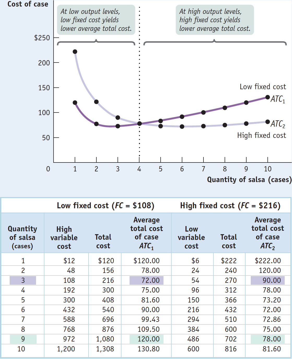
From the figure you can see that when output is small, 4 cases of salsa per day or fewer, average total cost is smaller when Selena forgoes the additional equipment and maintains the lower fixed cost of $108: ATC1 lies below ATC2. For example, at 3 cases per day, average total cost is $72 without the additional machinery and $90 with the additional machinery. But as output increases beyond 4 cases per day, the firm’s average total cost is lower if it acquires the additional equipment, raising its fixed cost to $216. For example, at 9 cases of salsa per day, average total cost is $120 when fixed cost is $108 but only $78 when fixed cost is $216.
Why does average total cost change like this when fixed cost increases? When output is low, the increase in fixed cost from the additional equipment outweighs the reduction in variable cost from higher worker productivity—
In general, for each output level there is some choice of fixed cost that minimizes the firm’s average total cost for that output level. So when the firm has a desired output level that it expects to maintain over time, it should choose the level of fixed cost optimal for that level—
Now that we are studying a situation in which fixed cost can change, we need to take time into account when discussing average total cost. All of the average total cost curves we have considered until now are defined for a given level of fixed cost—
For most firms, it is realistic to assume that there are many possible choices of fixed cost, not just two. The implication: for such a firm, many possible short-
At any given point in time, a firm will find itself on one of its short-
The long-
Suppose we do a thought experiment and calculate the lowest possible average total cost that can be achieved for each output level if the firm were to choose its fixed cost for each output level. Economists have given this thought experiment a name: the long-
11-12
Short-
We can now draw the distinction between the short run and the long run more fully. In the long run, when a producer has had time to choose the fixed cost appropriate for its desired level of output, that producer will be at some point on the long-
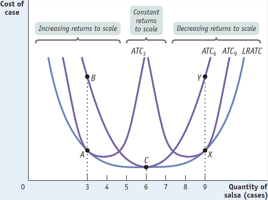
Figure 11-12 illustrates this point. The curve ATCļ shows short-
Suppose that Selena initially chose to be on ATC6. If she actually produces 6 cases of salsa per day, her firm will be at point C on both its short-
Suppose, conversely, that Selena ends up producing 9 cases per day even though she initially chose to be on ATC6. In the short run her average total cost is indicated by point Y on ATC6. But she would be better off purchasing more equipment and incurring a higher fixed cost in order to reduce her variable cost and move to ATC9. This would allow her to reach point X on the long-
The distinction between short-
Returns to Scale
There are increasing returns to scale when long-
What determines the shape of the long-
There are decreasing returns to scale when long-
As you can see in Figure 11-12, Selena’s Gourmet Salsas experiences increasing returns to scale over output levels ranging from 0 up to5 cases of salsa per day—
There are constant returns to scale when long-
There is also a third possible relationship between long-
What explains these scale effects in production? The answer ultimately lies in the firm’s technology of production. Increasing returns often arise from the increased specialization that larger output levels allow—
Another source of increasing returns is very large initial setup cost; in some industries—
A third source of increasing returns, found in certain high-
Decreasing returns—
Summing Up Costs: The Short and Long of It
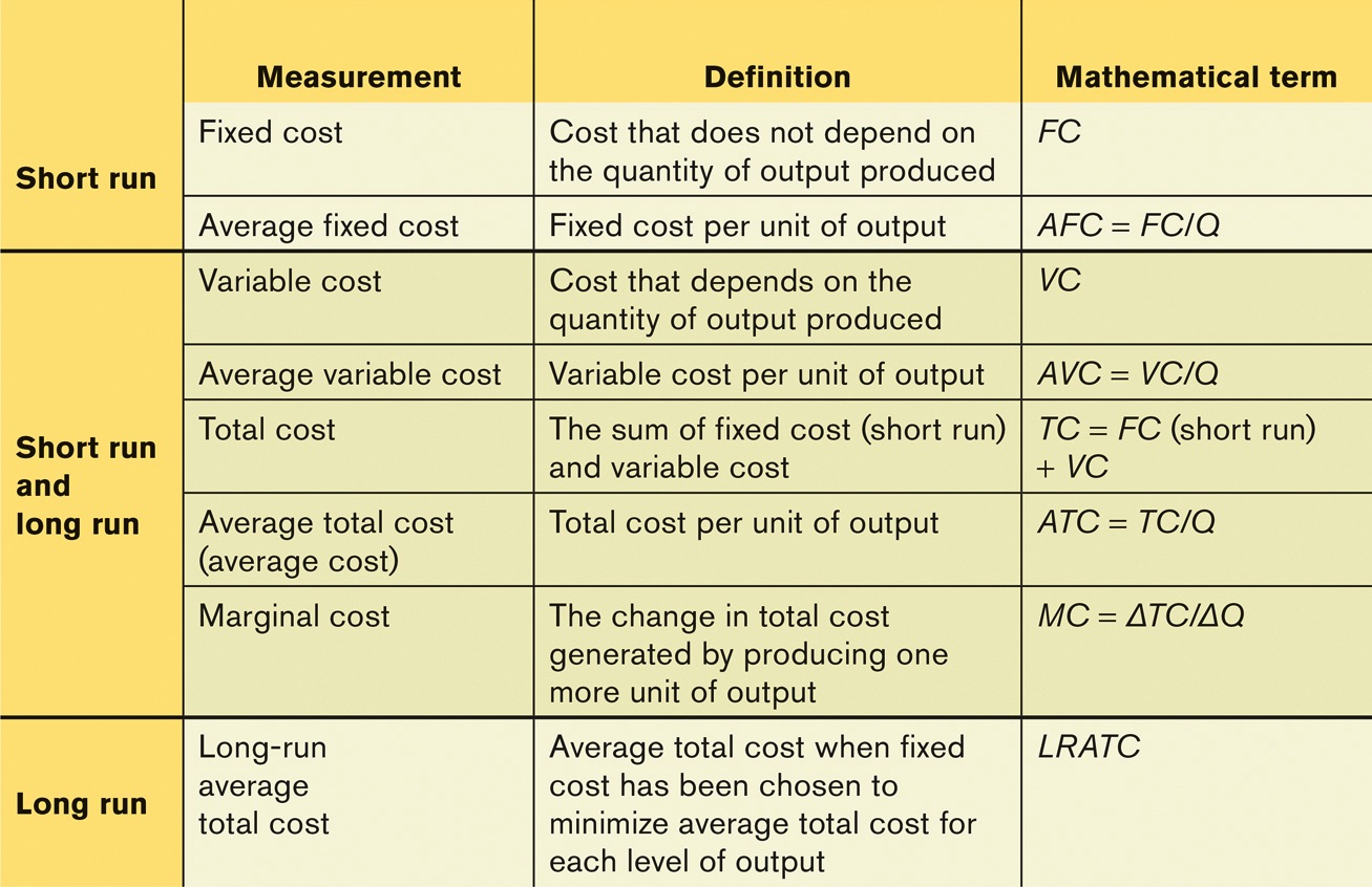
If a firm is to make the best decisions about how much to produce, it has to understand how its costs relate to the quantity of output it chooses to produce. Table 11-3 provides a quick summary of the concepts and measures of cost you have learned about.
11-3
Concepts and Measures of Cost
!worldview! ECONOMICS in Action: There’s No Business Like Snow Business
There’s No Business Like Snow Business
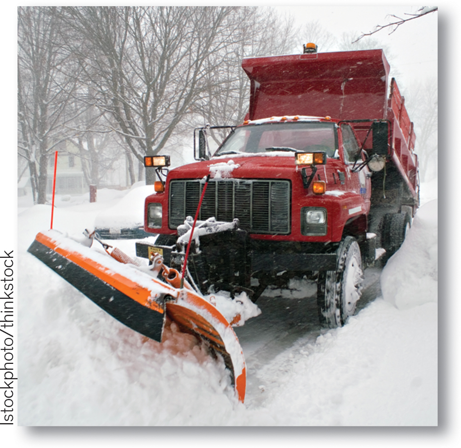
Anyone who has lived both in a snowy city, like Chicago, and in a city that only occasionally experiences significant snowfall, like Washington, D.C., is aware of the differences in total cost that arise from making different choices about fixed cost.
In Washington, even a minor snowfall—
In this sense Washington and Chicago are like two producers who expect to produce different levels of output, where the “output” is snow removal. Washington, which rarely has significant snow, has chosen a low level of fixed cost in the form of snow-
Quick Review
In the long run, firms choose fixed cost according to expected output. Higher fixed cost reduces average total cost when output is high. Lower fixed cost reduces average total cost when output is low.
There are many possible short-
run average total cost curves, each corresponding to a different level of fixed cost. The long- run average total cost curve, LRATC , shows average total cost over the long run, when the firm has chosen fixed cost to minimize average total cost for each level of output.A firm that has fully adjusted its fixed cost for its output level will operate at a point that lies on both its current short-
run and long- run average total cost curves. A change in output moves the firm along its current short- run average total cost curve. Once it has readjusted its fixed cost, the firm will operate on a new short- run average total cost curve and on the long- run average total cost curve. Scale effects arise from the technology of production. Increasing returns to scale tend to make firms larger. Decreasing returns to scale tend to limit their size. With constant returns to scale, scale has no effect.
11-3
Question 11.3
The accompanying table shows three possible combinations of fixed cost and average variable cost. Average variable cost is constant in this example (it does not vary with the quantity of output produced).
For each of the three choices, calculate the average total cost of producing 12,000, 22,000, and 30,000 units. For each of these quantities, which choice results in the lowest average total cost?
The accompanying table shows the average total cost of producing 12,000, 22,000, and 30,000 units for each of the three choices of fixed cost. For example, if the firm makes choice 1, the total cost of producing 12,000 units of output is $8,000 + 12,000 × $1.00 = $20,000. The average total cost of producing 12,000 units of output is therefore $20,000/12,000 = $1.67. The other average total costs are calculated similarly.12,000 units
22,000 units
30,000 units
Average total cost from choice 1
$1.67
$1.36
$1.27
Average total cost from choice 2
1.75
1.30
1.15
Average total cost from choice 3
2.25
1.34
1.05
So if the firm wanted to produce 12,000 units, it would make choice 1 because this gives it the lowest average total cost. If it wanted to produce 22,000 units, it would make choice 2. If it wanted to produce 30,000 units, it would make choice 3.
Suppose that the firm, which has historically produced 12,000 units, experiences a sharp, permanent increase in demand that leads it to produce 22,000 units. Explain how its average total cost will change in the short run and in the long run.
Choice
Fixed cost
Average variable cost
1
$8,000
$1.00
2
12,000
0.75
3
24,000
0.25
Having historically produced 12,000 units, the firm would have adopted choice 1. When producing 12,000 units, the firm would have had an average total cost of $1.67. When output jumps to 22,000 units, the firm cannot alter its choice of fixed cost in the short run, so its average total cost in the short run will be $1.36. In the long run, however, it will adopt choice 2, making its average total cost fall to $1.30.
Explain what the firm should do instead if it believes the change in demand is temporary.
If the firm believes that the increase in demand is temporary, it should not alter its fixed cost from choice 1 because choice 2 generates higher average total cost as soon as output falls back to its original quantity of 12,000 units: $1.75 versus $1.67.
Question 11.4
In each of the following cases, explain what kind of scale effects you think the firm will experience and why.
A telemarketing firm in which employees make sales calls using computers and telephones
This firm is likely to experience constant returns to scale. To increase output, the firm must hire more workers, purchase more computers, and pay additional telephone charges. Because these inputs are easily available, their long-run average total cost is unlikely to change as output increases.An interior design firm in which design projects are based on the expertise of the firm’s owner
This firm is likely to experience decreasing returns to scale. As the firm takes on more projects, the costs of communication and coordination required to implement the expertise of the firm’s owner are likely to increase. As a result, the firm’s long-run average total cost will increase as output increases.A diamond-
mining company This firm is likely to experience increasing returns to scale. Because diamond mining requires a large initial set-up cost for excavation equipment, long-run average total cost will fall as output increases.
Question 11.5
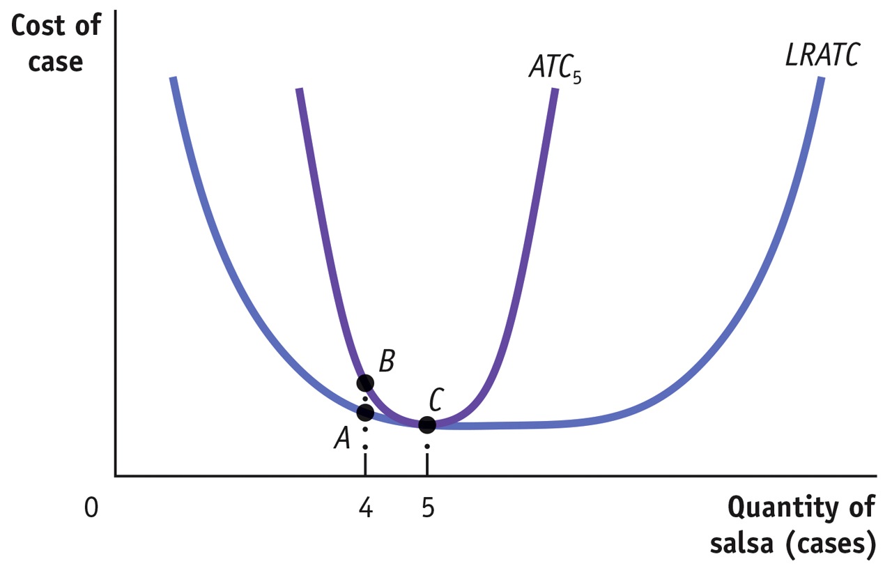
Draw a graph like Figure 11-12 and insert a short-
run average total cost curve corresponding to a long- run output choice of 5 cases of salsa per day. Use the graph to show why Selena should change her fixed cost if she expects to produce only 4 cases per day for a long period of time. The accompanying diagram shows the long-run average total cost curve (LRATC) and the short-run average total cost curve corresponding to a long-run output choice of 5 cases of salsa (ATC5). The curve ATC5 shows the short-run average total cost for which the level of fixed cost minimizes average total cost at an output of 5 cases of salsa. This is confirmed by the fact that at 5 cases per day, ATC5 touches LRATC, the long-run average total cost curve.
If Selena expects to produce only 4 cases of salsa for a long time, she should change her fixed cost. If she does not change her fixed cost and produces 4 cases of salsa, her average total cost in the short run is indicated by point B on ATC5; it is no longer on the LRATC. If she changes her fixed cost, though, her average total cost could be lower, at point A.
Solutions appear at back of book.
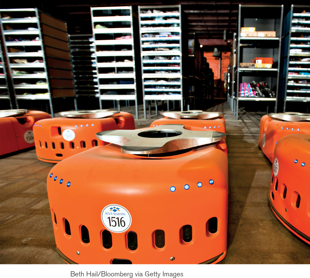
Kiva Systems’ Robots versus Humans: The Challenge of Holiday Order Fulfillment
For those who like to procrastinate when it comes to holiday shopping, the rise of e-
E-
Behind these technological advances, however, lies an intense debate: people versus robots. Amazon.com has relied on a large staff of temporary human workers to get it through the previous holiday seasons, often quadrupling its staff and operating 24 hours a day. In contrast, CrateandBarrel.com only doubled its workforce, thanks to a cadre of orange robots that allows each worker to do the work of six people.
But Amazon.com is set to increase its robotic work force in the future. In May 2012, Amazon.com bought Kiva Systems, the leader in order fulfillment robotics, for $775 million, with the hope of tailoring Kiva’s systems to fit Amazon.com’s warehouse and fulfillment needs.
Although many retailers—
As one industry analyst noted, an obstacle to the purchase of a robotic system for many e-
QUESTIONS FOR THOUGHT
Question 11.6
Assume that a firm can sell a robot, but that the sale takes time and the firm is likely to get less than what it paid. Other things equal, which system, human-
based or robotic, will have a higher fixed cost? Which will have a higher variable cost? Explain. Assume that a firm can sell a robot, but that the sale takes time and the firm is likely to get less than what it paid. Other things equal, which system, human-based or robotic, will have a higher fixed cost? Which will have a higher variable cost? Explain. Question 11.7
Predict the pattern of off-
holiday sales versus holiday sales that would induce a retailer to keep a human- based system. Predict the pattern that would induce a retailer to move to a robotic system. Predict the pattern of off-holiday sales versus holiday sales that would induce a retailer to keep a human- based system. Predict the pattern that would induce a retailer to move to a robotic system. Question 11.8
How would a “robot-
for- hire” program affect your answer to Question 2? Explain. How would a “robot-for- hire” program affect your answer to Question 2? Explain.