Production and Profits
Consider Noelle, who runs a Christmas tree farm. Suppose that the market price of Christmas trees is $18 per tree and that Noelle is a price-
12-1
Profit for Noelle’s Farm When Market Price Is $18
|
Quantity of trees Q |
Total revenue TR |
Total cost TC |
Profit TR − TC |
|---|---|---|---|
|
0 |
$0 |
$140 |
-$140 |
|
10 |
180 |
300 |
-120 |
|
20 |
360 |
360 |
0 |
|
30 |
540 |
440 |
100 |
|
40 |
720 |
560 |
160 |
|
50 |
900 |
720 |
180 |
|
60 |
1,080 |
920 |
160 |
|
70 |
1,260 |
1,160 |
100 |
TABLE 12-
The first column shows the quantity of output in number of trees, and the second column shows Noelle’s total revenue from her output: the market value of trees she produced. Total revenue, TR, is equal to the market price multiplied by the quantity of output:
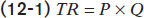
In this example, total revenue is equal to $18 per tree times the quantity of output in trees.
The third column of Table 12-1 shows Noelle’s total cost. The fourth column shows her profit, equal to total revenue minus total cost:

As indicated by the numbers in the table, profit is maximized at an output of 50 trees, where profit is equal to $180. But we can gain more insight into the profit-
Using Marginal Analysis to Choose the Profit-Maximizing Quantity of Output
Marginal revenue is the change in total revenue generated by an additional unit of output.
Recall from Chapter 9 the profit-

or
MR = ΔTR/ΔQ
According to the optimal output rule, profit is maximized by producing the quantity of output at which the marginal revenue of the last unit produced is equal to its marginal cost.
So Noelle maximizes her profit by producing trees up to the point at which the marginal revenue is equal to marginal cost. We can summarize this as the producer’s optimal output rule: profit is maximized by producing the quantity at which the marginal revenue of the last unit produced is equal to its marginal cost. That is, MR = MC at the optimal quantity of output.
We can learn how to apply the optimal output rule with the help of Table 12-2, which provides various short-
12-2
Short-Run Costs for Noelle’s Farm
The fifth column contains the farm’s marginal revenue, which has an important feature: Noelle’s marginal revenue equal to price is constant at $18 for every output level. The sixth and final column shows the calculation of the net gain per tree, which is equal to marginal revenue minus marginal cost—
According to the price-
This example, in fact, illustrates another general rule derived from marginal analysis—
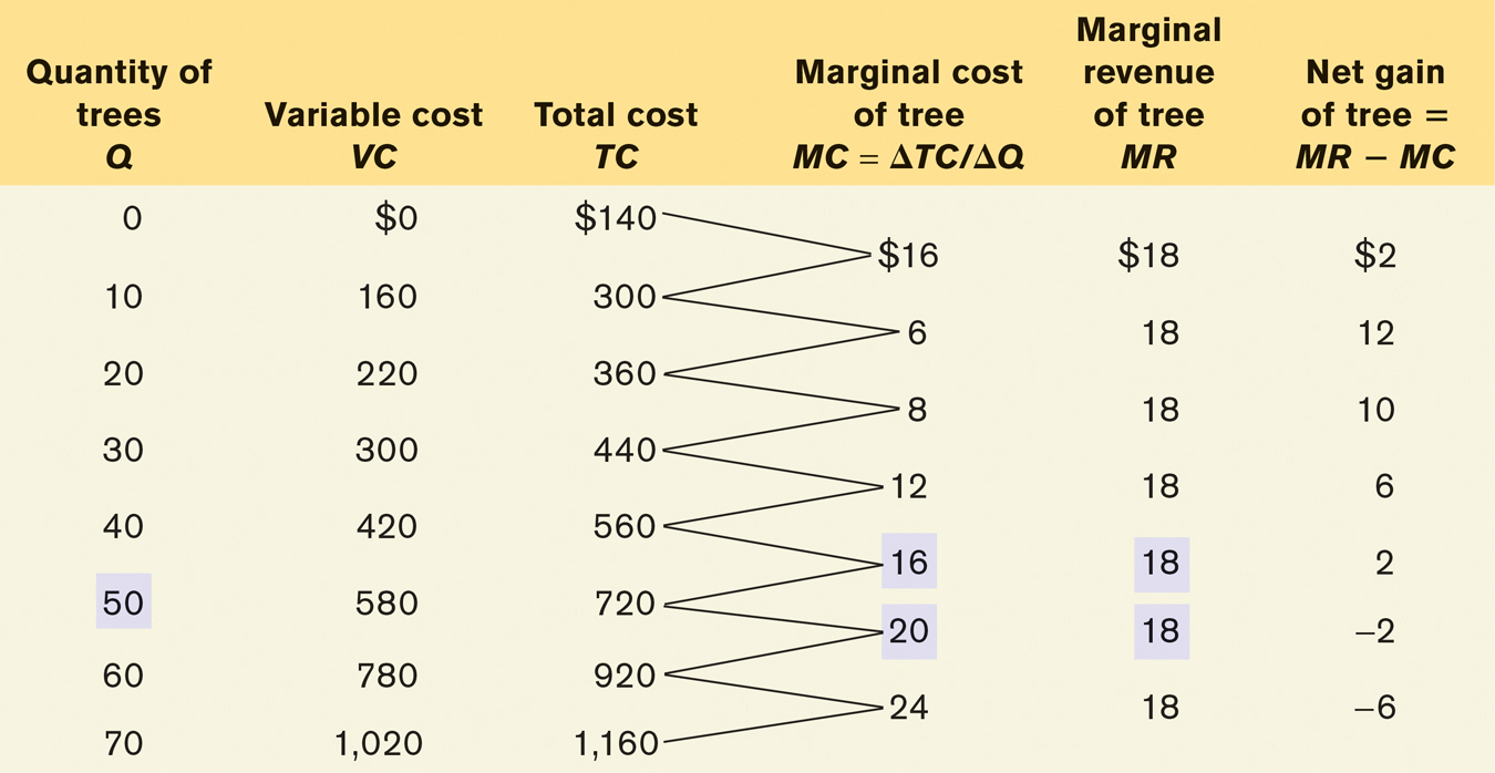
A price-
The marginal revenue curve shows how marginal revenue varies as output varies.
For the remainder of this chapter, we will assume that the industry in question is like Christmas tree farming, perfectly competitive. Figure 12-1 shows that Noelle’s profit-
12-1
The Price-
Note that whenever a firm is a price-
PITFALLS: WHAT IF MARGINAL REVENUE AND MARGINAL COST AREN’T EXACTLY EQUAL?
WHAT IF MARGINAL REVENUE AND MARGINAL COST AREN’T EXACTLY EQUAL?
The optimal output rule says that to maximize profit, you should produce the quantity at which marginal revenue is equal to marginal cost. But what do you do if there is no output level at which marginal revenue equals marginal cost? In that case, you produce the largest quantity for which marginal revenue exceeds marginal cost. This is the case in Table 12-2 at an output of 50 trees. The simpler version of the optimal output rule applies when production involves large numbers, such as hundreds or thousands of units. In such cases marginal cost comes in small increments, and there is always a level of output at which marginal cost almost exactly equals marginal revenue.
Does this mean that the price-
To understand why the first step in the production decision involves an “either–
When Is Production Profitable?
Recall from Chapter 9 that a firm’s decision whether or not to stay in a given business depends on its economic profit—the measure of profit based on the opportunity cost of resources used in the business. To put it a slightly different way: in the calculation of economic profit, a firm’s total cost incorporates the implicit cost—
In contrast, accounting profit is profit calculated using only the explicit costs incurred by the firm. This means that economic profit incorporates the opportunity cost of resources owned by the firm and used in the production of output, while accounting profit does not.
A firm may make positive accounting profit while making zero or even negative economic profit. It’s important to understand clearly that a firm’s decision to produce or not, to stay in business or to close down permanently, should be based on economic profit, not accounting profit.
So we will assume, as we always do, that the cost numbers given in Tables 12-1 and 12-2 include all costs, implicit as well as explicit, and that the profit numbers in Table 12-1 are therefore economic profit. So what determines whether Noelle’s farm earns a profit or generates a loss? The answer is that, given the farm’s cost curves, whether or not it is profitable depends on the market price of trees—
12-3
Short-Run Average Costs for Noelle’s Farm
|
Quantity of trees Q |
Variable cost VC |
Total cost TC |
Short- |
Short- |
|---|---|---|---|---|
|
10 |
$160.00 |
$300.00 |
$16.00 |
$30.00 |
|
20 |
220.00 |
360.00 |
11.00 |
18.00 |
|
30 |
300.00 |
440.00 |
10.00 |
14.67 |
|
40 |
420.00 |
560.00 |
10.50 |
14.00 |
|
50 |
580.00 |
720.00 |
11.60 |
14.40 |
|
60 |
780.00 |
920.00 |
13.00 |
15.33 |
|
70 |
1,020.00 |
1,160.00 |
14.57 |
16.57 |
TABLE 12-
In Table 12-3 we calculate short-
12-2
Costs and Production in the Short Run
To see how these curves can be used to decide whether production is profitable or unprofitable, recall that profit is equal to total revenue minus total cost, TR − TC. This means:
If the firm produces a quantity at which TR > TC, the firm is profitable.
If the firm produces a quantity at which TR = TC, the firm breaks even.
If the firm produces a quantity at which TR < TC, the firm incurs a loss.
We can also express this idea in terms of revenue and cost per unit of output. If we divide profit by the number of units of output, Q, we obtain the following expression for profit per unit of output:

TR/Q is average revenue, which is the market price. TC/Q is average total cost. So a firm is profitable if the market price for its product is more than the average total cost of the quantity the firm produces; a firm loses money if the market price is less than average total cost of the quantity the firm produces. This means:
If the firm produces a quantity at which P > ATC, the firm is profitable.
If the firm produces a quantity at which P = ATC, the firm breaks even.
If the firm produces a quantity at which P < ATC, the firm incurs a loss.
Figure 12-3 illustrates this result, showing how the market price determines whether a firm is profitable. It also shows how profits are depicted graphically. Each panel shows the marginal cost curve, MC, and the short-
12-3
Profitability and the Market Price
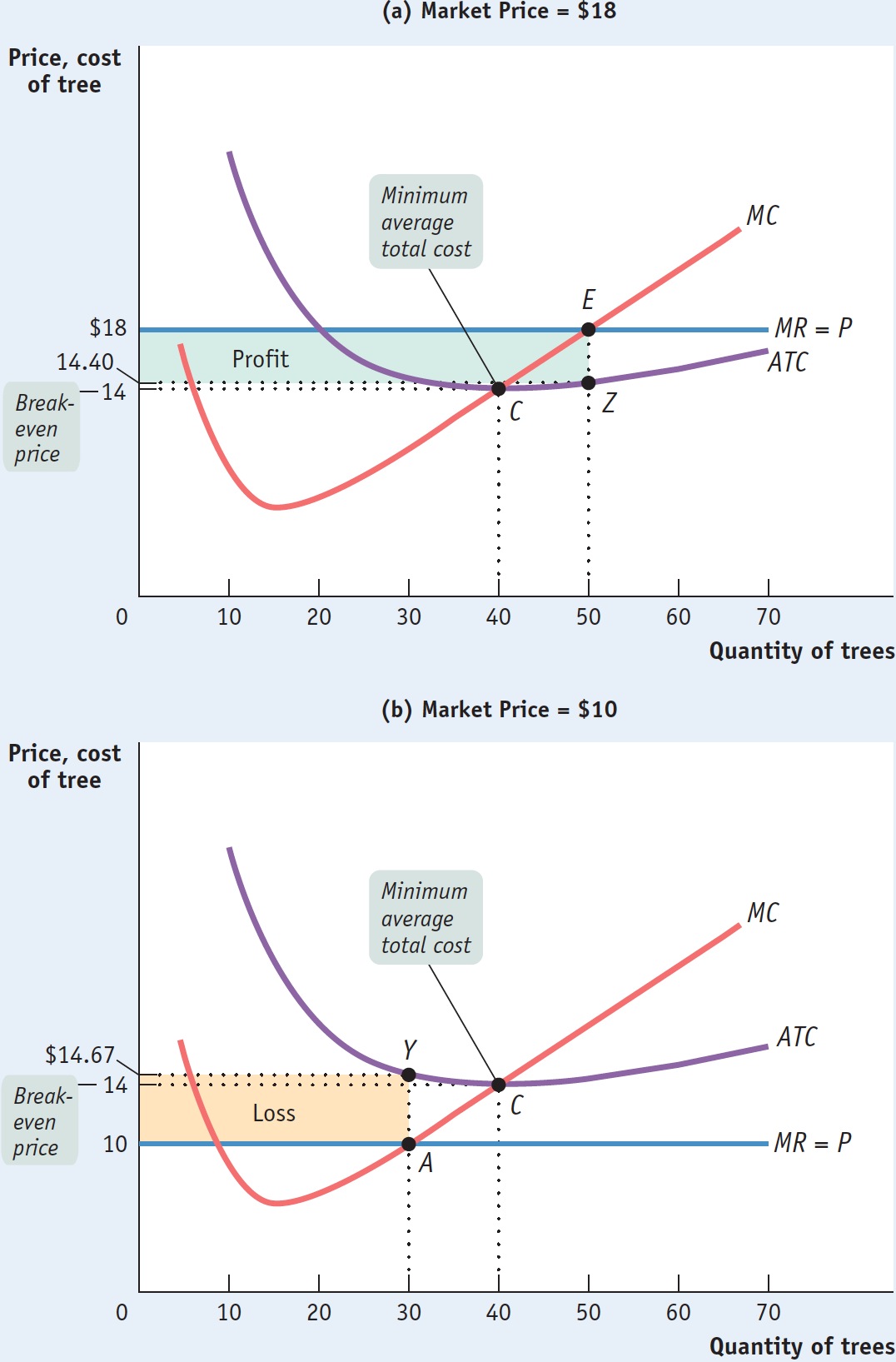
In panel (a), we see that at a price of $18 per tree the profit-
Noelle’s total profit when the market price is $18 is represented by the area of the shaded rectangle in panel (a). To see why, notice that total profit can be expressed in terms of profit per unit:

or, equivalently,
Profit = (P − ATC) × Q
since P is equal to TR/Q and ATC is equal to TC/Q. The height of the shaded rectangle in panel (a) corresponds to the vertical distance between points E and Z. It is equal to P − ATC = $18.00 − $14.40 = $3.60 per tree. The shaded rectangle has a width equal to the output: Q = 50 trees. So the area of that rectangle is equal to Noelle’s profit: 50 trees × $3.60 profit per tree = $180—
What about the situation illustrated in panel (b)? Here the market price of trees is $10 per tree. Setting price equal to marginal cost leads to a profit-
How much does she lose by producing when the market price is $10? On each tree she loses ATC − P = $14.67 − $10.00 = $4.67, an amount corresponding to the vertical distance between points A and Y. And she would produce 30 trees, which corresponds to the width of the shaded rectangle. So the total value of the losses is $4.67 × 30 = $140.00 (adjusted for rounding error), an amount that corresponds to the area of the shaded rectangle in panel (b).
But how does a producer know, in general, whether or not its business will be profitable? It turns out that the crucial test lies in a comparison of the market price to the producer’s minimum average total cost. On Noelle’s farm, minimum average total cost, which is equal to $14, occurs at an output quantity of 40 trees, indicated by point C.
Whenever the market price exceeds minimum average total cost, the producer can find some output level for which the average total cost is less than the market price. In other words, the producer can find a level of output at which the firm makes a profit. So Noelle’s farm will be profitable whenever the market price exceeds $14. And she will achieve the highest possible profit by producing the quantity at which marginal cost equals the market price.
Conversely, if the market price is less than minimum average total cost, there is no output level at which price exceeds average total cost. As a result, the firm will be unprofitable at any quantity of output. As we saw, at a price of $10—
The break-
The minimum average total cost of a price-
So the rule for determining whether a producer of a good is profitable depends on a comparison of the market price of the good to the producer’s breakeven price—
Whenever the market price exceeds minimum average total cost, the producer is profitable.
Whenever the market price equals minimum average total cost, the producer breaks even.
Whenever the market price is less than minimum average total cost, the producer is unprofitable.
The Short-Run Production Decision
You might be tempted to say that if a firm is unprofitable because the market price is below its minimum average total cost, it shouldn’t produce any output. In the short run, however, this conclusion isn’t right.
In the short run, sometimes the firm should produce even if price falls below minimum average total cost. The reason is that total cost includes fixed cost—cost that does not depend on the amount of output produced and can only be altered in the long run.
In the short run, fixed cost must still be paid, regardless of whether or not a firm produces. For example, if Noelle rents a refrigerated truck for the year, she has to pay the rent on the truck regardless of whether she produces any trees. Since it cannot be changed in the short run, her fixed cost is irrelevant to her decision about whether to produce or shut down in the short run.
Although fixed cost should play no role in the decision about whether to produce in the short run, other costs—
Let’s turn to Figure 12-4: it shows both the short-
12-4
The Short-
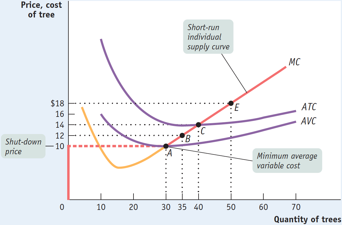
Because the marginal cost curve has a “swoosh” shape—
We are now prepared to fully analyze the optimal production decision in the short run. We need to consider two cases:
When the market price is below minimum average variable cost
When the market price is greater than or equal to minimum average variable cost
When the market price is below minimum average variable cost, the price the firm receives per unit is not covering its variable cost per unit. A firm in this situation should cease production immediately. Why? Because there is no level of output at which the firm’s total revenue covers its variable costs—
A firm will cease production in the short run if the market price falls below the shut-
In this case the firm maximizes its profits by not producing at all—
When price is greater than minimum average variable cost, however, the firm should produce in the short run. In this case, the firm maximizes profit—
But what if the market price lies between the shut-
Yet even if it isn’t covering its total cost per unit, it is covering its variable cost per unit and some—
This means that whenever price lies between minimum average total cost and minimum average variable cost, the firm is better off producing some output in the short run. The reason is that by producing, it can cover its variable cost per unit and at least some of its fixed cost, even though it is incurring a loss. In this case, the firm maximizes profit—
It’s worth noting that the decision to produce when the firm is covering its variable costs but not all of its fixed cost is similar to the decision to ignore sunk costs. You may recall from Chapter 9 that a sunk cost is a cost that has already been incurred and cannot be recouped; and because it cannot be changed, it should have no effect on any current decision.
In the short-
And what happens if market price is exactly equal to the shut-
The short-
Putting everything together, we can now draw the short-
As long as the market price is equal to or above the shut-
Do firms really shut down temporarily without going out of business? Yes. In fact, in some businesses temporary shut-
Changing Fixed Cost
Although fixed cost cannot be altered in the short run, in the long run firms can acquire or get rid of machines, buildings, and so on. As we learned in Chapter 11, in the long run the level of fixed cost is a matter of choice. There we saw that a firm will choose the level of fixed cost that minimizes the average total cost for its desired output quantity. Now we will focus on an even bigger question facing a firm when choosing its fixed cost: whether to incur any fixed cost at all by remaining in its current business.
In the long run, a producer can always eliminate fixed cost by selling off its plant and equipment. If it does so, of course, it can’t ever produce—
Consider Noelle’s farm once again. In order to simplify our analysis, we will sidestep the problem of choosing among several possible levels of fixed cost. Instead, we will assume from now on that Noelle has only one possible choice of fixed cost if she operates, the amount of $140, Noelle’s minimum average total cost, that was the basis for the calculations in Tables 12-1, 12-2, and 12-3. (With this assumption, Noelle’s short-
Suppose that the market price of trees is consistently less than $14 over an extended period of time. In that case, Noelle never fully covers her fixed cost: her business runs at a persistent loss. In the long run, then, she can do better by closing her business and leaving the industry. In other words, in the long run firms will exit an industry if the market price is consistently less than their break-
Conversely, suppose that the price of Christmas trees is consistently above the break-
But things won’t stop there. The Christmas tree industry meets the criterion of free entry: there are many potential tree producers because the necessary inputs are easy to obtain. And the cost curves of those potential producers are likely to be similar to those of Noelle, since the technology used by other producers is likely to be very similar to that used by Noelle. If the price is high enough to generate profits for existing producers, it will also attract some of these potential producers into the industry. So in the long run a price in excess of $14 should lead to entry: new producers will come into the Christmas tree industry.
As we will see next, exit and entry lead to an important distinction between the short-
Summing Up: The Perfectly Competitive Firm’s Profitability and Production Conditions
In this chapter, we’ve studied where the supply curve for a perfectly competitive, price-
12-4
Summary of the Perfectly Competitive Firm’s Profitability and Production Conditions
|
Profitability condition (minimum ATC = break- |
Result |
|
P > minimum ATC |
Firm profitable. Entry into industry in the long run. |
|
P = minimum ATC |
Firm breaks even. No entry into or exit from industry in the long run. |
|
P < minimum ATC |
Firm unprofitable. Exit from industry in the long run. |
|
Production condition (minimum AVC = shut- |
Result |
|
P > minimum AVC |
Firm produces in the short run. If P < minimum ATC, firm covers variable cost and some but not all of fixed cost. If P > minimum ATC, firm covers all variable cost and fixed cost. |
|
P = minimum AVC |
Firm indifferent between producing in the short run or not. Just covers variable cost. |
|
P < minimum AVC |
Firm shuts down in the short run. Does not cover variable cost. |
TABLE 12-
!worldview! ECONOMICS in Action: Farmers Move Up Their Supply Curves
Farmers Move Up Their Supply Curves
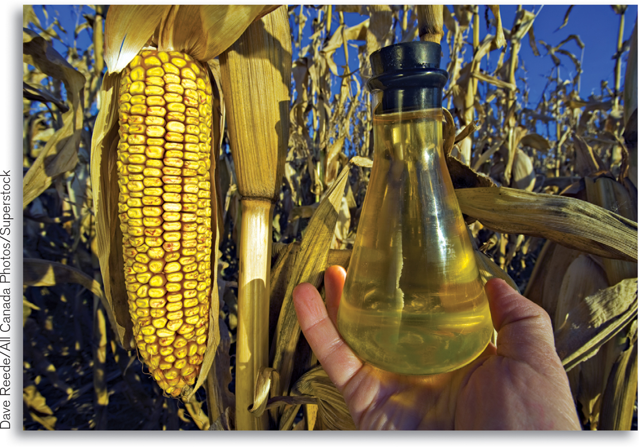
To reduce gasoline consumption, Congress mandated that increasing amounts of biofuel, mostly corn-
If this sounds like a sure way to make a profit, think again. Corn farmers were taking a considerable gamble in planting more corn as their costs went up. Consider the cost of fertilizer, an important input. Corn requires more fertilizer than other crops, and with more farmers planting corn, the increased demand for fertilizer led to a price increase. In 2006 and 2007, fertilizer prices surged to five times their 2005 level; by 2013 prices were still twice as high.
The pull of higher corn prices also lifted farmland prices to record levels—
Despite the risk and increase in costs, what corn farmers did made complete economic sense. By planting more corn, each farmer moved up his or her individual supply curve. And because the individual supply curve is the marginal cost curve, each farmer’s costs also went up because of the need to use more inputs that are now more expensive to obtain.
So the moral of the story is that farmers will increase their corn acreage until the marginal cost of producing corn is approximately equal to the market price of corn—
Quick Review
A producer chooses output according to the optimal output rule. For a price-
taking firm, marginal revenue is equal to price and it chooses output according to the price- taking firm’s optimal output rule P = MC .A firm is profitable whenever price exceeds its break-
even price , equal to its minimum average total cost. Below that price it is unprofitable. It breaks even when price is equal to its break-even price. Fixed cost is irrelevant to the firm’s optimal short-
run production decision. When price exceeds its shut- down price , minimum average variable cost, the price-taking firm produces the quantity of output at which marginal cost equals price. When price is lower than its shut- down price, it ceases production in the short run. This defines the firm’s short- run individual supply curve .Over time, fixed cost matters. If price consistently falls below minimum average total cost, a firm will exit the industry. If price exceeds minimum average total cost, the firm is profitable and will remain in the industry; other firms will enter the industry in the long run.
12-2
Question 12.2
Draw a short-
run diagram showing a U- shaped average total cost curve, a U- shaped average variable cost curve, and a “swoosh”-shaped marginal cost curve. On it, indicate the range of output and the range of price for which the following actions are optimal. The firm shuts down immediately.
The firm should shut down immediately when price is less than minimum average variable cost, the shut-down price. In the accompanying diagram, this is optimal for prices in the range 0 to P1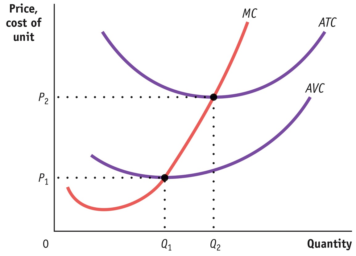
The firm operates in the short run despite sustaining a loss.
When price is greater than minimum average variable cost (the shut-down price) but less than minimum average total cost (the break-even price), the firm should continue to operate in the short run even though it is making a loss. This is optimal for prices in the range P1 to P2 and for quantities Q1 to Q2.The firm operates while making a profit.
When price exceeds minimum average total cost (the break-even price), the firm makes a profit. This happens for prices in excess of P2 and results in quantities greater than Q2.
Question 12.3
The state of Maine has a very active lobster industry, which harvests lobsters during the summer months. During the rest of the year, lobsters can be obtained from other parts of the world but at a much higher price. Maine is also full of “lobster shacks,” roadside restaurants serving lobster dishes that are open only during the summer. Explain why it is optimal for lobster shacks to operate only during the summer.
This is an example of a temporary shut-down by a firm when the market price lies below the shut-down price, the minimum average variable cost. In this case, the market price is the price of a lobster meal and variable cost is the variable cost of serving such a meal, such as the cost of the lobster, employee wages, and so on. In this example, however, it is the average variable cost curve rather than the market price that shifts over time, due to seasonal changes in the cost of lobsters. Maine lobster shacks have relatively low average variable cost during the summer, when cheap Maine lobsters are available. During the rest of the year, their average variable cost is relatively high due to the high cost of imported lobsters. So the lobster shacks are open for business during the summer, when their minimum average variable cost lies below price. But they close during the rest of the year, when price lies below their minimum average variable cost.
Solutions appear at back of book.