Understanding Monopolistic Competition
Suppose an industry is monopolistically competitive: it consists of many producers, all competing for the same consumers but offering differentiated products. How does such an industry behave?
As the term monopolistic competition suggests, this market structure combines some features typical of monopoly with others typical of perfect competition. Because each firm is offering a distinct product, it is in a way like a monopolist: it faces a downward-
The same, of course, is true of an oligopoly. In a monopolistically competitive industry, however, there are many producers, as opposed to the small number that defines an oligopoly. This means that the “puzzle” of oligopoly—
But such collusion is virtually impossible when the number of firms is large and, by implication, there are no barriers to entry. So in situations of monopolistic competition, we can safely assume that firms behave noncooperatively and ignore the potential for collusion.
Monopolistic Competition in the Short Run
We introduced the distinction between short-
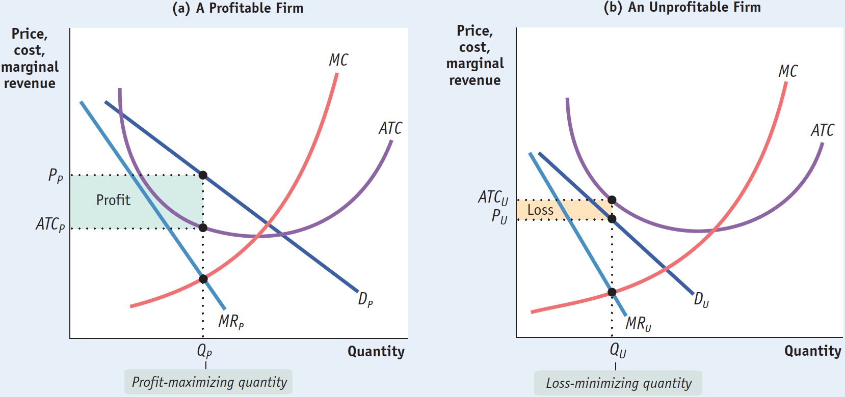
Panels (a) and (b) of Figure 15-1 show two possible situations that a typical firm in a monopolistically competitive industry might face in the short run. In each case, the firm looks like any monopolist: it faces a downward-
15-1
The Monopolistically Competitive Firm in the Short Run

We assume that every firm has an upward-
In each case the firm, in order to maximize profit, sets marginal revenue equal to marginal cost. So how do these two figures differ? In panel (a) the firm is profitable; in panel (b) it is unprofitable. (Recall that we are referring always to economic profit, not accounting profit—
In panel (a) the firm faces the demand curve DP and the marginal revenue curve MRP. It produces the profit-
In panel (b) the firm faces the demand curve DU and the marginal revenue curve MRU. It chooses the quantity QU at which marginal revenue is equal to marginal cost. However, in this case the price PU is below the average total cost ATCU; so at this quantity the firm loses money. Its loss is equal to the area of the shaded rectangle. Since QU is the profit-
As this comparison suggests, the key to whether a firm with market power is profitable or unprofitable in the short run lies in the relationship between its demand curve and its average total cost curve. In panel (a) the demand curve DP crosses the average total cost curve, meaning that some of the demand curve lies above the average total cost curve. So there are some price-
In panel (b), by contrast, the demand curve DU does not cross the average total cost curve—
These figures, showing firms facing downward-
Monopolistic Competition in the Long Run
Obviously, an industry in which existing firms are losing money, like the one in panel (b) of Figure 15-1, is not in long-
It may be less obvious that an industry in which existing firms are earning profits, like the one in panel (a) of Figure 15-1, is also not in long-
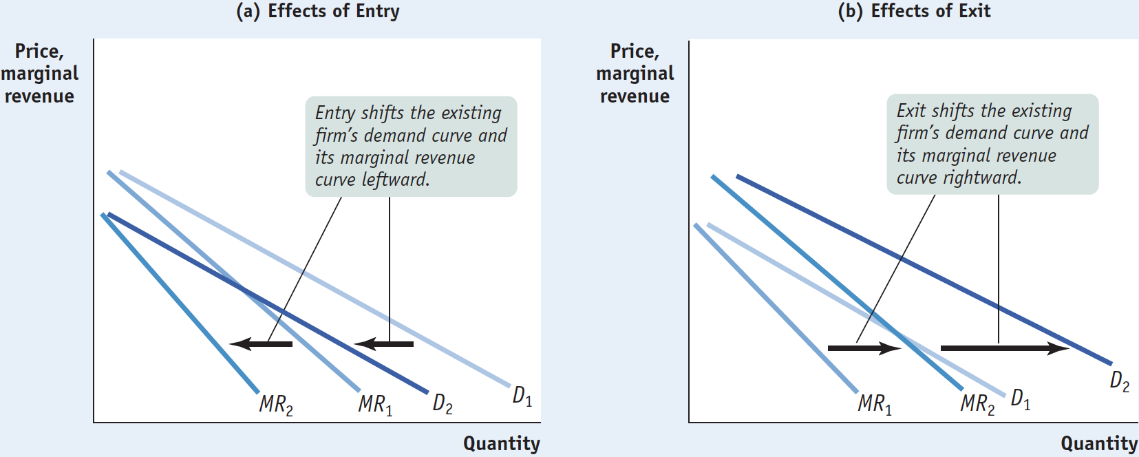
How will entry or exit by other firms affect the profits of a typical existing firm? Because the differentiated products offered by firms in a monopolistically competitive industry compete for the same set of customers, entry or exit by other firms will affect the demand curve facing every existing producer. If new gas stations open along a highway, each of the existing gas stations will no longer be able to sell as much gas as before at any given price. So, as illustrated in panel (a) of Figure 15-2, entry of additional producers into a monopolistically competitive industry will lead to a leftward shift of the demand curve and the marginal revenue curve facing a typical existing producer.
15-2
Entry and Exit Shift Existing Firm’s Demand Curve and Marginal Revenue Curve

Conversely, suppose that some of the gas stations along the highway close. Then each of the remaining stations will be able to sell more gasoline at any given price. So, as illustrated in panel (b), exit of firms from an industry will lead to a rightward shift of the demand curve and marginal revenue curve facing a typical remaining producer.
In the long run, a monopolistically competitive industry ends up in zero-
The industry will be in long-
We have seen that a firm facing a downward-
If this is not the case, the firm operating at its profit-
Hits and Flops
On the face of it, the movie business seems to meet the criteria for monopolistic competition. Movies compete for the same consumers; each movie is different from the others; new companies can and do enter the business. But where’s the zero-
The key is to realize that for every successful blockbuster, there are several flops—
The difference between movie-
Yet there is still, in a way, a zero-
In fact, as you might expect, the movie industry on average earns just about enough to cover the cost of production—
This kind of situation—
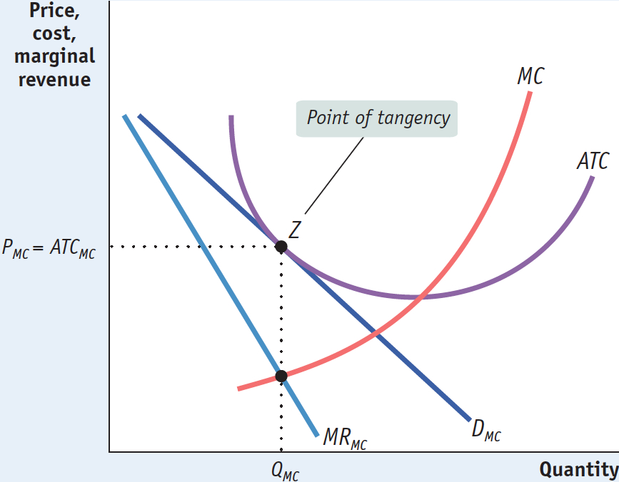
Figure 15-3 shows a typical monopolistically competitive firm in such a zero-
15-3
The Long-

The normal long-
ECONOMICS in Action: The Housing Bust and the Demise of the 6% Commission
The Housing Bust and the Demise of the 6% Commission
The vast majority of home sales in the United States are transacted with the use of real estate agents. A home owner looking to sell hires an agent, who lists the house for sale and shows it to interested buyers. Correspondingly, prospective home buyers hire their own agent to arrange inspections of available houses. Traditionally, agents were paid by the seller: a commission equal to 6% of the sales price of the house, which the seller’s agent and the buyer’s agent would split equally. If a house sold for $300,000, for example, the seller’s agent and the buyer’s agent each received $9,000 (equal to 3% of $300,000).
The real estate brokerage industry fits the model of monopolistic competition quite well: in any given local market, there are many real estate agents, all competing with one another, but the agents are differentiated by location and personality as well as by the type of home they sell (some focus on condominiums, others on very expensive homes, and so on). And the industry has free entry: it’s relatively easy for someone to become a real estate agent (take a course and then pass a test to obtain a license).
But for a long time there was one feature that didn’t fit the model of monopolistic competition: the fixed 6% commission that had not changed over time and was unaffected by the ups and downs of the housing market. How could this be? Why didn’t new agents enter the market and drive the commission down to the zero-
One tactic used by agents was their control of the Multiple Listing Service, or MLS, which lists nearly all the homes for sale in a community. Traditionally, only sellers who agreed to the 6% commission were allowed to list homes on the MLS.
But protecting the 6% commission was always an iffy endeavor because any action by the brokerage industry to fix the commission rate at a given percentage would run afoul of antitrust laws. And by the early to mid-
Oversight by regulators and the housing market bust which began in 2006 hastened the demise of the non-
Quick Review
Like a monopolist, each firm in a monopolistically competitive industry faces a downward-
sloping demand curve and marginal revenue curve. In the short run, it may earn a profit or incur a loss at its profit- maximizing quantity. If the typical firm earns positive profit, new firms will enter the industry in the long run, shifting each existing firm’s demand curve to the left. If the typical firm incurs a loss, some existing firms will exit the industry in the long run, shifting the demand curve of each remaining firm to the right.
The long-
run equilibrium of a monopolistically competitive industry is a zero- profit equilibrium in which firms just break even. The typical firm’s demand curve is tangent to its average total cost curve at its profit-maximizing quantity.
15-2
Question 15.3
Currently a monopolistically competitive industry, composed of firms with U-
shaped average total cost curves, is in long- run equilibrium. Describe how the industry adjusts, in both the short and long run, in each of the following situations. A technological change that increases fixed cost for every firm in the industry
An increase in fixed cost raises average total cost and shifts the average total cost curve upward. In the short run, firms incur losses. In the long run, some will exit the industry, resulting in a rightward shift of the demand curves for those firms that remain in the industry, since each one now serves a larger share of the market. Long-run equilibrium is reestablished when the demand curve for each remaining firm has shifted rightward to the point where it is tangent to the firm’s new, higher average total cost curve. At this point each firm’s price just equals its average total cost, and each firm makes zero profit.A technological change that decreases marginal cost for every firm in the industry
A decrease in marginal cost lowers average total cost and shifts the average total cost curve and the marginal cost curve downward. Because existing firms now make profits, in the long run new entrants are attracted into the industry. In the long run, this results in a leftward shift of each existing firm’s demand curve since each firm now has a smaller share of the market. Long-run equilibrium is reestablished when each firm’s demand curve has shifted leftward to the point where it is tangent to the new, lower average total cost curve. At this point each firm’s price just equals average total cost, and each firm makes zero profit.
Question 15.4
Why, in the long run, is it impossible for firms in a monopolistically competitive industry to create a monopoly by joining together to form a single firm?
If all the existing firms in the industry joined together to create a monopoly, they would achieve monopoly profits. But this would induce new firms to create new, differentiated products and then enter the industry and capture some of the monopoly profits. So in the long run it would be impossible to maintain a monopoly. The problem arises from the fact that because new firms can create new products, there is no barrier to entry that can maintain a monopoly.
Solutions appear at back of book.