Depending on his tastes, Clive’s utility-maximizing choice of hours of leisure and income could lie anywhere on the time allocation budget line in Figure 19A-1. Let’s assume that his optimal choice is point A, at which he consumes 40 hours of leisure and earns $400. Now we are ready to link the analysis of time allocation to labor supply.

When Clive chooses a point like A on his time allocation budget line, he is also choosing the quantity of labor he supplies to the labor market. By choosing to consume 40 of his 80 available hours as leisure, he has also chosen to supply the other 40 hours as labor.

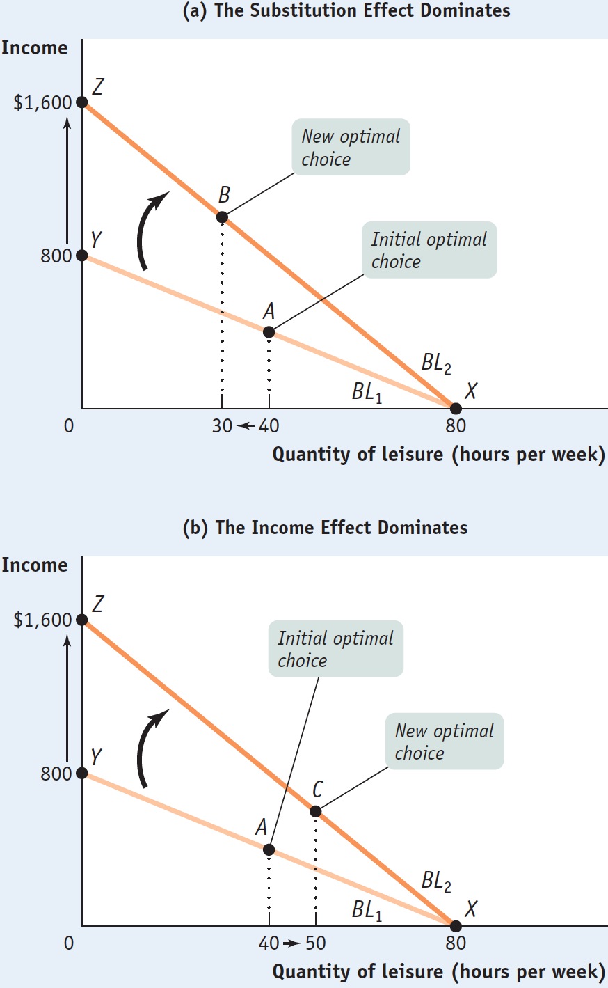
Now suppose that Clive’s wage rate doubles, from $10 to $20 per hour. The effect of this increase in his wage rate is shown in Figure 19A-2. His time allocation budget line rotates outward: the vertical intercept, which represents the amount he could earn if he devoted all 80 hours to work, shifts upward from point Y to point Z. As a result of the doubling of his wage, Clive would earn $1,600 instead of $800 if he devoted all 80 hours to working.

But how will Clive’s time allocation actually change? As we saw in the chapter, this depends on the income effect and substitution effect that we learned about in Chapter 10 and its appendix.

The substitution effect of an increase in the wage rate works as follows. When the wage rate increases, the opportunity cost of an hour of leisure increases; this induces Clive to consume less leisure and work more hours—that is, to substitute hours of work in place of hours of leisure as the wage rate rises. If the substitution effect were the whole story, the individual labor supply curve would look like any ordinary supply curve and would always slope upward—a higher wage rate leads to a greater quantity of labor supplied.

What we learned in our analysis of demand was that for most consumer goods, the income effect isn’t very important because most goods account for only a very small share of a consumer’s spending. In addition, in the few cases of goods where the income effect is significant—for example, major purchases like housing—it usually reinforces the substitution effect: most goods are normal goods, so when a price increase makes a consumer poorer, he or she buys less of that good.

In the labor/leisure choice, however, the income effect takes on a new significance, for two reasons. First, most people get the great majority of their income from wages. This means that the income effect of a change in the wage rate is not small: an increase in the wage rate will generate a significant increase in income. Second, leisure is a normal good: when income rises, other things equal, people tend to consume more leisure and work fewer hours.

So the income effect of a higher wage rate tends to reduce the quantity of labor supplied, working in opposition to the substitution effect, which tends to increase the quantity of labor supplied. So the net effect of a higher wage rate on the quantity of labor Clive supplies could go either way—depending on his preferences, he might choose to supply more labor, or he might choose to supply less labor. The two panels of Figure 19A-2 illustrate these two outcomes. In each panel, point A represents Clive’s initial consumption choice. Panel (a) shows the case in which Clive works more hours in response to a higher wage rate. An increase in the wage rate induces him to move from point A to point B, where he consumes less leisure than at A and therefore works more hours. Here the substitution effect prevails over the income effect. Panel (b) shows the case in which Clive works fewer hours in response to a higher wage rate. Here, he moves from point A to point C, where he consumes more leisure and works fewer hours than at A. Here the income effect prevails over the substitution effect.

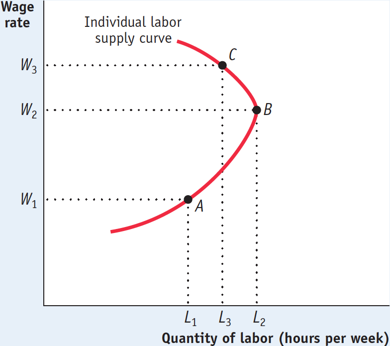
When the income effect of a higher wage rate is stronger than the substitution effect, the individual labor supply curve, which shows how much labor an individual will supply at any given wage rate will have a segment that slopes the “wrong” way—downward: a higher wage rate leads to a smaller quantity of labor supplied. An example is the segment connecting points B and C in Figure 19A-3.

Economists believe that the substitution effect usually dominates the income effect in the labor supply decision when an individual’s wage rate is low. An individual labor supply curve typically slopes upward for lower wage rates as people work more in response to rising wage rates. But they also believe that many individuals have stronger preferences for leisure and will choose to cut back the number of hours worked as their wage rate continues to rise. For these individuals, the income effect eventually dominates the substitution effect as the wage rate rises, leading their individual labor supply curves to change slope and to “bend backward” at high wage rates. An individual labor supply curve with this feature, called a backward-bending individual labor supply curve, is shown in Figure 19A-3. Although an individual labor supply curve may bend backward, market labor supply curves almost always slope upward over their entire range as higher wage rates draw more new workers into the labor market.