Changes in Supply and Demand
The huge fall in the price of natural gas from $14 to $2 per BTU from 2006 to 2013 may have come as a surprise to consumers, but to suppliers it was no surprise at all. Suppliers knew that advances in drilling technology had opened up vast reserves of natural gas that had been too costly to tap in the past. And, predictably, an increase in supply reduces the equilibrium price.
The adoption of improved drilling technology is an example of an event that shifted the supply curve for a good without having an effect on the demand curve. There are many such events. There are also events that shift the demand curve without shifting the supply curve. For example, a medical report that chocolate is good for you increases the demand for chocolate but does not affect the supply. Events often shift either the supply curve or the demand curve, but not both; it is therefore useful to ask what happens in each case.
We have seen that when a curve shifts, the equilibrium price and quantity change. We will now concentrate on exactly how the shift of a curve alters the equilibrium price and quantity.
What Happens When the Demand Curve Shifts
Heating oil and natural gas are substitutes: if the price of heating oil rises, the demand for natural gas will increase, and if the price of heating oil falls, the demand for natural gas will decrease. But how does the price of heating oil affect the market equilibrium for natural gas?
Figure 3-14 shows the effect of a rise in the price of heating oil on the market for natural gas. The rise in the price of heating oil increases the demand for natural gas. Point E1 shows the equilibrium corresponding to the original demand curve, with P1 the equilibrium price and Q1 the equilibrium quantity bought and sold.
3-14
Equilibrium and Shifts of the Demand Curve
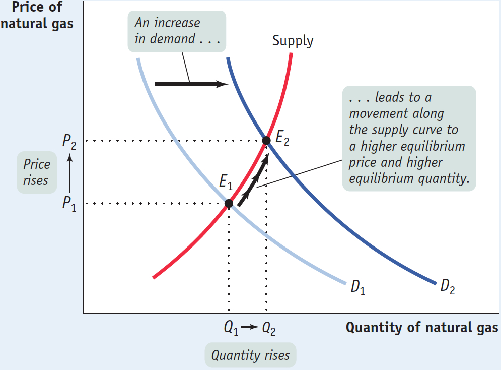
An increase in demand is indicated by a rightward shift of the demand curve from D1 to D2. At the original market price P1, this market is no longer in equilibrium: a shortage occurs because the quantity demanded exceeds the quantity supplied. So the price of natural gas rises and generates an increase in the quantity supplied, an upward movement along the supply curve. A new equilibrium is established at point E2, with a higher equilibrium price, P2, and higher equilibrium quantity, Q2. This sequence of events reflects a general principle: When demand for a good or service increases, the equilibrium price and the equilibrium quantity of the good or service both rise.
What would happen in the reverse case, a fall in the price of heating oil? A fall in the price of heating oil reduces the demand for natural gas, shifting the demand curve to the left. At the original price, a surplus occurs as quantity supplied exceeds quantity demanded. The price falls and leads to a decrease in the quantity supplied, resulting in a lower equilibrium price and a lower equilibrium quantity. This illustrates another general principle: When demand for a good or service decreases, the equilibrium price and the equilibrium quantity of the good or service both fall.
To summarize how a market responds to a change in demand: An increase in demand leads to a rise in both the equilibrium price and the equilibrium quantity. A decrease in demand leads to a fall in both the equilibrium price and the equilibrium quantity.
What Happens When the Supply Curve Shifts
For most goods and services, it is a bit easier to predict changes in supply than changes in demand. Physical factors that affect supply, like weather or the availability of inputs, are easier to get a handle on than the fickle tastes that affect demand. Still, with supply as with demand, what we can best predict are the effects of shifts of the supply curve.
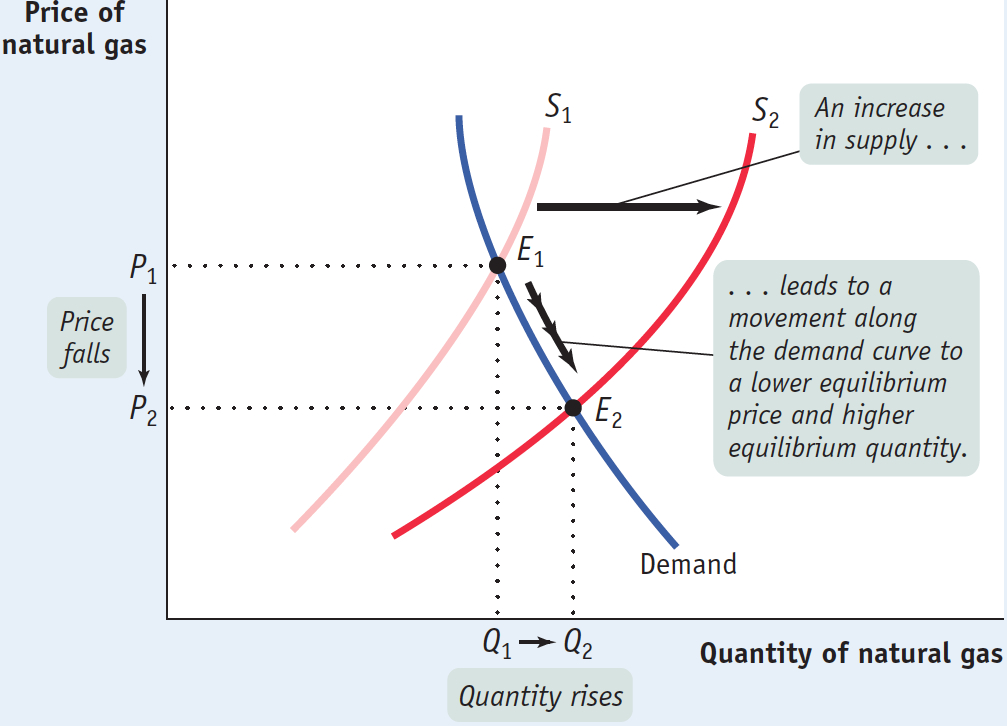
As we mentioned in the opening story, improved drilling technology significantly increased the supply of natural gas from 2006 onward. Figure 3-15 shows how this shift affected the market equilibrium. The original equilibrium is at E1, the point of intersection of the original supply curve, S1, with an equilibrium price P1 and equilibrium quantity Q1. As a result of the improved technology, supply increases and S1 shifts rightward to S2. At the original price P1, a surplus of natural gas now exists and the market is no longer in equilibrium. The surplus causes a fall in price and an increase in the quantity demanded, a downward movement along the demand curve. The new equilibrium is at E2, with an equilibrium price P2 and an equilibrium quantity Q2. In the new equilibrium E2, the price is lower and the equilibrium quantity is higher than before. This can be stated as a general principle: When supply of a good or service increases, the equilibrium price of the good or service falls and the equilibrium quantity of the good or service rises.
3-15
Equilibrium and Shifts of the Supply Curve
PITFALLS: WHICH CURVE IS IT, ANYWAY?
WHICH CURVE IS IT, ANYWAY?
When the price of some good or service changes, in general, we can say that this reflects a change in either supply or demand. But it is easy to get confused about which one. A helpful clue is the direction of change in the quantity. If the quantity sold changes in the same direction as the price—
What happens to the market when supply falls? A fall in supply leads to a leftward shift of the supply curve. At the original price a shortage now exists; as a result, the equilibrium price rises and the quantity demanded falls. This describes what happened to the market for natural gas after Hurricane Katrina damaged natural gas production in the Gulf of Mexico in 2006. We can formulate a general principle: When supply of a good or service decreases, the equilibrium price of the good or service rises and the equilibrium quantity of the good or service falls.
To summarize how a market responds to a change in supply: An increase in supply leads to a fall in the equilibrium price and a rise in the equilibrium quantity. A decrease in supply leads to a rise in the equilibrium price and a fall in the equilibrium quantity.
Simultaneous Shifts of Supply and Demand Curves
Finally, it sometimes happens that events shift both the demand and supply curves at the same time. This is not unusual; in real life, supply curves and demand curves for many goods and services shift quite often because the economic environment continually changes. Figure 3-16 illustrates two examples of simultaneous shifts. In both panels there is an increase in supply—
3-16
Simultaneous Shifts of the Demand and Supply Curves
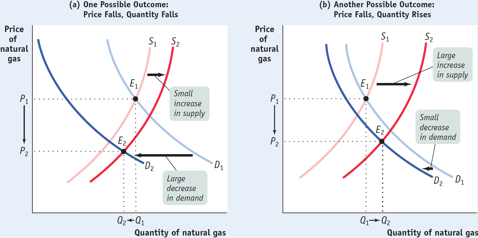
In both cases the equilibrium price falls from P1 to P2 as the equilibrium moves from E1 to E2. But what happens to the equilibrium quantity, the quantity of natural gas bought and sold? In panel (a) the decrease in demand is large relative to the increase in supply, and the equilibrium quantity falls as a result. In panel (b) the increase in supply is large relative to the decrease in demand, and the equilibrium quantity rises as a result. That is, when demand decreases and supply increases, the actual quantity bought and sold can go either way depending on how much the demand and supply curves have shifted.
Tribulations on the Runway
You probably don’t spend much time worrying about the trials and tribulations of fashion models. Most of them don’t lead glamorous lives; in fact, except for a lucky few, life as a fashion model today can be very trying and not very lucrative. And it’s all because of supply and demand.
Consider the case of Bianca Gomez, a willowy 18-
But once in New York, Bianca entered the global market for fashion models. And it wasn’t very pretty. Due to the ease of transmitting photos electronically and the relatively low cost of international travel, top fashion centers such as New York and Milan, Italy, are deluged each year with thousands of beautiful young women from all over the world, eagerly trying to make it as models. Although Russians, other Eastern Europeans, and Brazilians are particularly numerous, some hail from places such as Kazakhstan and Mozambique.

Returning to our (less glamorous) economic model of supply and demand, the influx of aspiring fashion models from around the world can be represented by a rightward shift of the supply curve in the market for fashion models, which would by itself tend to lower the price paid to models.
And that wasn’t the only change in the market. Unfortunately for Bianca and others like her, the tastes of many of those who hire models have changed as well. Fashion magazines have come to prefer using celebrities such as Beyoncé on their pages rather than anonymous models, believing that their readers connect better with a familiar face. This amounts to a leftward shift of the demand curve for models—
This was borne out in Bianca’s experiences. After paying her rent, her transportation, all her modeling expenses, and 20% of her earnings to her modeling agency (which markets her to prospective clients and books her jobs), Bianca found that she was barely breaking even. Sometimes she even had to dip into savings from her high school years. To save money, she ate macaroni and hot dogs; she traveled to auditions, often four or five in one day, by subway. As the Wall Street Journal reported, Bianca was seriously considering quitting modeling altogether.
In general, when supply and demand shift in opposite directions, we can’t predict what the ultimate effect will be on the quantity bought and sold. What we can say is that a curve that shifts a disproportionately greater distance than the other curve will have a disproportionately greater effect on the quantity bought and sold. That said, we can make the following prediction about the outcome when the supply and demand curves shift in opposite directions:
When demand decreases and supply increases, the equilibrium price falls but the change in the equilibrium quantity is ambiguous.
When demand increases and supply decreases, the equilibrium price rises but the change in the equilibrium quantity is ambiguous.
But suppose that the demand and supply curves shift in the same direction. This is what has happened in recent years in the United States, as the economy has made a gradual recovery from the recession of 2008, resulting in an increase in both demand and supply. Can we safely make any predictions about the changes in price and quantity? In this situation, the change in quantity bought and sold can be predicted, but the change in price is ambiguous. The two possible outcomes when the supply and demand curves shift in the same direction (which you should check for yourself) are as follows:
When both demand and supply increase, the equilibrium quantity rises but the change in equilibrium price is ambiguous.
When both demand and supply decrease, the equilibrium quantity falls but the change in equilibrium price is ambiguous.
!worldview! ECONOMICS in Action: The Cotton Panic and Crash of 2011
The Cotton Panic and Crash of 2011
When fear of a future price increase strikes a large enough number of consumers, it can become a self-
The process had, in fact, been started by real events that occurred years earlier. By 2010, demand for cotton had rebounded sharply from lows set during the global financial crisis of 2006-
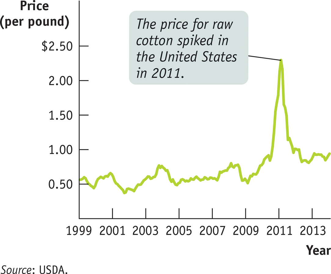
3-17
Cotton Prices in the United States, 1999–
At the same time there were significant supply reductions to the worldwide market for cotton. India, the second largest exporter of cotton (an exporter is a seller of a good to foreign buyers), had imposed restrictions on the sale of its cotton abroad in order to aid its own textile mills. And Pakistan, China, and Australia, which were big growers of cotton, experienced widespread flooding that significantly reduced their cotton crops. The Indian export restrictions and the floods in cotton-
So, as shown in Figure 3-17, while cotton had traded at between $0.35 and $0.60 per pound from 2000 to 2010, it surged to more than $2.40 per pound in early 2011—
Yet by the end of 2011, cotton prices had plummeted to $0.86 per pound. What happened? A number of things, illustrating the forces of supply and demand. First, demand fell as clothing manufacturers, unwilling to pass on huge price increases to their customers, shifted to less expensive fabrics like polyester. Second, supply increased as farmers planted more acreage of cotton in hopes of garnering high prices. As the effects of supply and demand became obvious, buyers stopped panicking and cotton prices finally fell back down to earth.
Quick Review
Changes in the equilibrium price and quantity in a market result from shifts of the supply curve, the demand curve, or both.
An increase in demand increases both the equilibrium price and the equilibrium quantity. A decrease in demand decreases both the equilibrium price and the equilibrium quantity.
An increase in supply drives the equilibrium price down but increases the equilibrium quantity. A decrease in supply raises the equilibrium price but reduces the equilibrium quantity.
Often fluctuations in markets involve shifts of both the supply and demand curves. When they shift in the same direction, the change in equilibrium quantity is predictable but the change in equilibrium price is not. When they shift in opposite directions, the change in equilibrium price is predictable but the change in equilibrium quantity is not. When there are simultaneous shifts of the demand and supply curves, the curve that shifts the greater distance has a greater effect on the change in equilibrium price and quantity.
3-4
Question 3.4
In each of the following examples, determine (i) the market in question; (ii) whether a shift in demand or supply occurred, the direction of the shift, and what induced the shift; and (iii) the effect of the shift on the equilibrium price and the equilibrium quantity.
As the price of gasoline fell in the United States during the 1990s, more people bought large cars.
The market for large cars: this is a rightward shift in demand caused by a decrease in the price of a complement, gasoline. As a result of the shift, the equilibrium price of large cars will rise and the equilibrium quantity of large cars bought and sold will also rise.As technological innovation has lowered the cost of recycling used paper, fresh paper made from recycled stock is used more frequently.
The market for fresh paper made from recycled stock: this is a rightward shift in supply due to a technological innovation. As a result of this shift, the equilibrium price of fresh paper made from recycled stock will fall and the equilibrium quantity bought and sold will rise.When a local cable company offers cheaper on-
demand films, local movie theaters have more unfilled seats. The market for movies at a local movie theater: this is a leftward shift in demand caused by a fall in the price of a substitute, on-demand films. As a result of this shift, the equilibrium price of movie tickets will fall and the equilibrium number of people who go to the movies will also fall.
Question 3.5
When a new, faster computer chip is introduced, demand for computers using the older, slower chips decreases. Simultaneously, computer makers increase their production of computers containing the old chips in order to clear out their stocks of old chips.
Draw two diagrams of the market for computers containing the old chips:
one in which the equilibrium quantity falls in response to these events and
Upon the announcement of the new chip, the demand curve for computers using the earlier chip shifts leftward, as demand decreases, and the supply curve for these computers shifts rightward, as supply increases.
If demand decreases relatively more than supply increases, then the equilibrium quantity falls, as shown here:
one in which the equilibrium quantity rises.
If supply increases relatively more than demand decreases, then the equilibrium quantity rises, as shown here: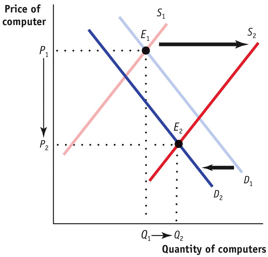
What happens to the equilibrium price in each diagram?
In both cases, the equilibrium price falls.
Solutions appear at back of book.