1.2 57The Market for Loanable Funds

WHAT YOU WILL LEARN
 How the loanable funds market matches savers and investors
 The determinants of supply and demand in the loanable funds market
 How changes in the expected future inflation rate affect the nominal interest rate
The Role of the Loanable Funds Market
For the economy as a whole, savings always equals investment spending. In a closed economy, savings is equal to national savings. In an open economy, savings is equal to national savings plus capital inflow. At any given time, however, savers, the people with funds to lend, are usually not the same as borrowers, the people who want to borrow to finance their investment spending. How are savers and borrowers brought together?
Savers and borrowers are matched up with one another in much the same way producers and consumers are matched up: through markets governed by supply and demand. In Figure 46-2, the expanded circular-
The loanable funds market is a hypothetical market that illustrates the market outcome of the demand for funds generated by borrowers and the supply of funds provided by lenders.
Although there are a large number of different financial markets in the financial system, such as the bond market and the stock market, economists often work with a simplified model in which they assume that there is just one market. The market brings together those who want to lend money (savers) and those who want to borrow (firms with investment spending projects). This hypothetical market is known as the loanable funds market.
The price that is determined in the loanable funds market is the interest rate, denoted by r. As we’ve learned, loans typically specify a nominal interest rate. So although we call r “the interest rate,” it is with the understanding that r is a nominal interest rate—
In the interest of simplicity we are also going to assume that there is only one type of loan. This, despite the fact that in reality there are many different kinds of interest rates because there are many different kinds of loans—
Now we’re ready to analyze how savings and investment get matched up.
The Demand for Loanable Funds
Figure 57-1 illustrates a hypothetical demand curve for loanable funds, D, which slopes downward. On the horizontal axis we show the quantity of loanable funds demanded. On the vertical axis we show the interest rate, which is the “price” of borrowing. But why does the demand curve for loanable funds slope downward?

To answer this question, consider what a firm is doing when it engages in investment spending—

So an investment is worth making only if it generates a future return that is greater than the monetary cost of making the investment today. How much greater? To answer that, we need to take into account the present value of the future return the firm expects to get.
We will look at the concept of present value in more detail in the next module. For now, keep in mind that in present value calculations, we use the interest rate to determine how the value of a dollar in the future compares to the value of a dollar today. But the fact is that future dollars are worth less than a dollar today, and they are worth even less when the interest rate is higher.
The intuition behind present value calculations is simple. The interest rate measures the opportunity cost of investment spending that results in a future return: instead of spending money on an investment spending project, a company could simply put the money into the bank and earn interest on it. And the higher the interest rate, the more attractive it is to simply put money into the bank instead of investing it in an investment spending project. In other words, the higher the interest rate, the higher the opportunity cost of investment spending. And, the higher the opportunity cost of investment spending, the lower the number of investment spending projects firms want to carry out, and therefore the lower the quantity of loanable funds demanded. It is this insight that explains why the demand curve for loanable funds is downward sloping.
When businesses engage in investment spending, they spend money right now in return for an expected payoff in the future. So, to evaluate whether a particular investment spending project is worth undertaking, a business must compare the present value of the future payoff with the current cost of that project. If the present value of the future payoff is greater than the current cost, a project is profitable and worth investing in. If the interest rate falls, then the present value of any given project rises, so more projects pass that test. If the interest rate rises, then the present value of any given project falls, so fewer projects pass that test.
So total investment spending, and therefore the demand for loanable funds to finance that spending, is negatively related to the interest rate. Thus, the demand curve for loanable funds slopes downward. You can see this in Figure 57-1. When the interest rate falls from 12% to 4%, the quantity of loanable funds demanded rises from $150 billion (point A) to $450 billion (point B).
The Supply of Loanable Funds
Figure 57-2 shows a hypothetical supply curve for loanable funds, S. Again, the interest rate plays the same role that the price plays in ordinary supply and demand analysis. But why is this curve upward sloping?


The answer is that loanable funds are supplied by savers, and savers incur an opportunity cost when they lend to a business: the funds could instead be spent on consumption—
So it is a good assumption that more people will forgo current consumption and make a loan to a borrower when the interest rate is higher. As a result, our hypothetical supply curve of loanable funds slopes upward. In Figure 57-2, lenders will supply $150 billion to the loanable funds market at an interest rate of 4% (point X); if the interest rate rises to 12%, the quantity of loanable funds supplied will rise to $450 billion (point Y).
The Equilibrium Interest Rate
The interest rate at which the quantity of loanable funds supplied equals the quantity of loanable funds demanded is the equilibrium interest rate. As you can see in Figure 57-3, the equilibrium interest rate, r*, and the total quantity of lending, Q*, are determined by the intersection of the supply and demand curves, at point E. Here, the equilibrium interest rate is 8%, at which $300 billion is lent and borrowed. In this equilibrium, only investment spending projects that are profitable if the interest rate is 8% or higher are funded.
Projects that are profitable only when the interest rate falls below 8% are not funded. Correspondingly, only lenders who are willing to accept an interest rate of 8% or less will have their offers to lend funds accepted; lenders who demand an interest rate higher than 8% do not have their offers to lend accepted.
Figure 57-3 shows how the market for loanable funds matches up desired savings with desired investment spending: in equilibrium, the quantity of funds that savers want to lend is equal to the quantity of funds that firms want to borrow. The figure also shows that this match-

The insight that the loanable funds market leads to an efficient use of savings, although drawn from a highly simplified model, has important implications for real life: it is the reason that a well-
Let’s look at how the market for loanable funds responds to shifts of demand and supply. As in the standard model of supply and demand, where the equilibrium price changes in response to shifts of the demand or supply curves, here the equilibrium interest rate changes when there are shifts of the demand curve for loanable funds, the supply curve for loanable funds, or both.
Shifts of the Demand for Loanable Funds
Let’s start by looking at the causes and effects of changes in demand.
The factors that can cause the demand curve for loanable funds to shift include the following:
- Changes in perceived business opportunities. A change in beliefs about the payoff of investment spending can increase or reduce the amount of desired spending at any given interest rate. If there is great excitement over the business possibilities created by new technology, as there was when the Internet came into wide use in the 1990s, businesses will rush to buy computer equipment, put fiber-
optic cables in the ground, and so on, shifting the demand for loanable funds to the right. But if there is disillusionment with technology- related investment, as there was in 2001 when many dot- com businesses failed, the demand for loanable funds will shift back to the left. - Changes in government borrowing. A government runs a budget deficit when, in a given year, it spends more than it receives. Running budget deficits can be a major source of demand for loanable funds, with the result that changes in the government budget deficit can shift the demand curve for loanable funds. For example, between 2000 and 2003, as the U.S. federal government went from a budget surplus to a budget deficit, the government went from being a net saver that provided loanable funds to the market to being a net borrower, borrowing funds from the market. In 2000, net federal borrowing was minus $189 billion, as the federal government was paying off some of its pre-
existing debt. But by 2003, net federal borrowing was plus $416 billion because the government had to borrow large sums to pay its bills. This change had the effect, other things equal, of shifting the demand curve for loanable funds to the right.
Figure 57-4 shows the effects of an increase in the demand for loanable funds. S is the supply of loanable funds, and D1 is the initial demand curve. The initial equilibrium interest rate is r1. An increase in the demand for loanable funds means that the quantity of funds demanded rises at any given interest rate, so the demand curve shifts rightward to D2. As a result, the equilibrium interest rate rises to r2.

The fact that an increase in the demand for loanable funds leads, other things equal, to a rise in the interest rate has one especially important implication: it tells us that increasing or persistent government budget deficits are cause for concern because an increase in the government’s deficit shifts the demand curve for loanable funds to the right, which leads to a higher interest rate. If the interest rate rises, businesses will cut back on their investment spending.
Crowding out occurs when a government budget deficit drives up the interest rate and leads to reduced investment spending.
So, other things equal, a rise in the government budget deficit tends to reduce overall investment spending. Economists call the negative effect of government budget deficits on investment spending crowding out. Concerns about crowding out are one key reason to worry about increasing or persistent budget deficits.
However, it’s important to add a qualification here: crowding out may not occur if the economy is depressed. When the economy is operating far below full employment, government spending can lead to higher incomes; and these higher incomes lead to increased savings at any given interest rate. Higher savings allows the government to borrow without raising interest rates. Many economists believe, for example, that the large budget deficits that the U.S. government ran from 2008 to 2013, in the face of a depressed economy, caused little if any crowding out.
Shifts of the Supply of Loanable Funds
Like the demand for loanable funds, the supply of loanable funds can shift. Among the factors that can cause the supply of loanable funds to shift are the following:
- Changes in private savings behavior. A number of factors can cause the level of private savings to change at any given interest rate. For example, rising home prices in the United States will make many homeowners feel richer, leading them to spend more and save less. This will have the effect of shifting the supply curve of loanable funds to the left.
- Changes in net capital inflows. Capital flows into and out of a country can change as investors’ perceptions of that country change. For example, Greece experienced large net capital inflows after the creation of the euro, Europe’s common currency, in 1999, because investors believed that Greece’s adoption of the euro as its currency had made it a safe place to put their funds. But, in the years that followed, worries about the Greek government’s solvency (and the discovery that it had been understating its debt) led to a collapse in investor confidence, and the net inflow of funds dried up. The effect of shrinking capital inflows was to shift the supply curve in the Greek loanable funds market to the left.
Figure 57-5 shows the effects of an increase in the supply of loanable funds. D is the demand for loanable funds, and S1 is the initial supply curve. The initial equilibrium interest rate is r1. An increase in the supply of loanable funds means that the quantity of funds supplied rises at any given interest rate, so the supply curve shifts rightward to S2. As a result, the equilibrium interest rate falls to r2.

Inflation and Interest Rates
Anything that shifts either the supply of loanable funds curve or the demand for loanable funds curve changes the interest rate. Historically, major changes in interest rates have been driven by many factors, including changes in government policy and technological innovations that created new investment opportunities.
However, arguably the most important factor affecting interest rates over time—
To understand the effect of expected future inflation on interest rates, let’s look at an example: in the 1970s and 1980s higher than expected U.S. inflation reduced the real value of homeowners’ mortgages, which was good for the homeowners but bad for the banks. Economists summarize the effect of inflation on borrowers and lenders by distinguishing between the nominal interest rate and the real interest rate, where the difference is:
Real interest rate = Nominal interest rate − Inflation rate
The true cost of borrowing is the real interest rate, not the nominal interest rate.
To see why, suppose a firm borrows $10,000 for one year at a 10% nominal interest rate. At the end of the year, it must repay $11,000—
Similarly, the true payoff to lending is the real interest rate, not the nominal rate. Suppose that a bank makes a $10,000 loan for one year at a 10% nominal interest rate. At the end of the year, the bank receives an $11,000 repayment. But if the average level of prices rises by 10% per year, the purchasing power of the money the bank gets back is no more than that of the money it lent out. In real terms, the bank has made a zero-
Now we can add an important detail to our analysis of the loanable funds market. Figures 57-4 and 57-5 are drawn with the vertical axis measuring the nominal interest rate for a given expected future inflation rate. Why do we use the nominal interest rate rather than the real interest rate? Because in the real world neither borrowers nor lenders know what the future inflation rate will be when they make a deal.
Actual loan contracts therefore specify a nominal interest rate rather than a real interest rate. Because we are holding the expected future inflation rate fixed in Figures 57-4 and 57-5, however, changes in the nominal interest rate also lead to changes in the real interest rate.
The expectations of borrowers and lenders about future inflation rates are normally based on recent experience. In the late 1970s, after a decade of high inflation, borrowers and lenders expected future inflation to be high. By the late 1990s, after a decade of fairly low inflation, borrowers and lenders expected future inflation to be low.

These changing expectations about future inflation had a strong effect on the nominal interest rate, largely explaining why nominal interest rates were much lower in the early years of the twenty-
In Figure 57-6, the curves S0 and D0 show the supply and demand for loanable funds given that the expected future rate of inflation is 0%. In that case, equilibrium is at E0 and the equilibrium nominal interest rate is 4%. Because expected future inflation is 0%, the equilibrium expected real interest rate over the life of the loan is also 4%.

Now suppose that the expected future inflation rate rises to 10%. The demand curve for loanable funds shifts upward to D10: borrowers are now willing to borrow as much at a nominal interest rate of 14% as they were previously willing to borrow at 4%. That’s because with a 10% inflation rate, a 14% nominal interest rate corresponds to a 4% real interest rate.
Similarly, the supply curve of loanable funds shifts upward to S10: lenders require a nominal interest rate of 14% to persuade them to lend as much as they would previously have lent at 4%. The new equilibrium is at E10: the result of an expected future inflation rate of 10% is that the equilibrium nominal interest rate rises from 4% to 14%.
According to the Fisher effect, an increase in expected future inflation drives up the nominal interest rate, leaving the expected real interest rate unchanged.
This situation can be summarized as a general principle, known as the Fisher effect, which states that the expected real interest rate is unaffected by changes in expected future inflation. According to the Fisher effect, an increase in expected future inflation drives up the nominal interest rate, where each additional percentage point of expected future inflation drives up the nominal interest rate by 1 percentage point.
The central point is that both lenders and borrowers base their decisions on the expected real interest rate. As a result, a change in the expected rate of inflation does not affect the equilibrium quantity of loanable funds or the expected real interest rate; all it affects is the equilibrium nominal interest rate.
FIFTY YEARS OF FLUCTUATIONS IN U.S. INTEREST RATES
There have been some large movements in U.S. interest rates over the past half-
Panel (a) of Figure 57-7 illustrates the first effect. It shows the average interest rate on bonds issued by the U.S. government—

It’s not hard to see why that happened: inflation shot up during the 1970s, leading to widespread expectations that high inflation would continue. And as we’ve seen, expected inflation raises the equilibrium interest rate. As inflation came down in the 1980s, so did expectations of future inflation, and this brought interest rates down as well.
Panel (b) illustrates the second effect: changes in the expected return on investment spending and interest rates, with a “close-
What happened, instead, was the boom and bust in housing: interest rates rose as demand for housing soared, pushing the demand curve for loanable funds to the right, then fell as the housing boom collapsed, shifting the demand curve for loanable funds back to the left. Throughout this whole process, total savings was equal to total investment spending, and the rise and fall of the interest rate played a key role in matching lenders with borrowers.
57
Solutions appear at the back of the book.
Check Your Understanding
Use a diagram of the loanable funds market to illustrate the effect of the following events on the equilibrium interest rate and investment spending.
-
a. An economy is opened to international movements of capital, and a net capital inflow occurs.
As capital flows into the economy, the supply of loanable funds increases. This is illustrated by the shift of the supply curve from S1 to S2 in the accompanying diagram. As the equilibrium moves from E1 to E2, the equilibrium interest rate falls from r1 to r2, and the equilibrium quantity of loanable funds increases from Q1 to Q2.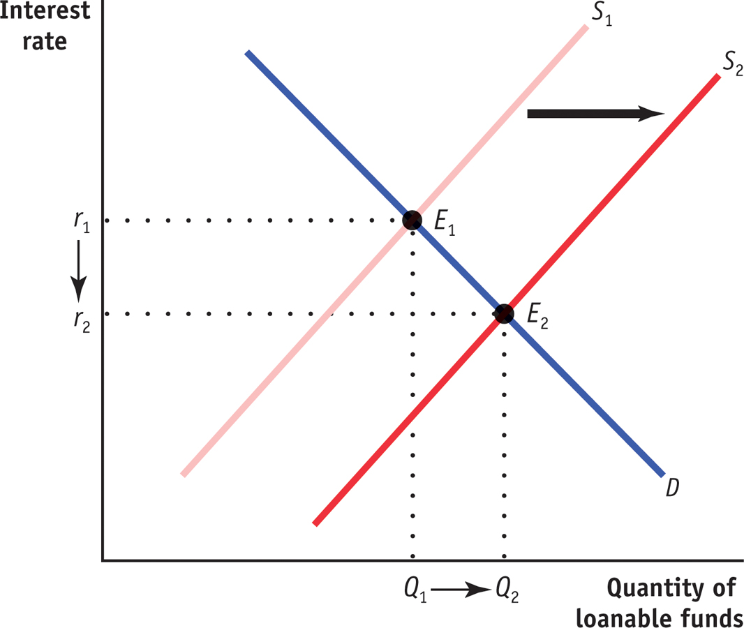
-
b. Retired people generally save less than working people at any interest rate. The proportion of retired people in the population goes up.
Savings fall due to the higher proportion of retired people, and the supply of loanable funds decreases. This is illustrated by the leftward shift of the supply curve from S1 to S2 in the accompanying diagram. The equilibrium moves from E1 to E2, the equilibrium interest rate rises from r1 to r2, and the equilibrium quantity of loanable funds falls from Q1 to Q2.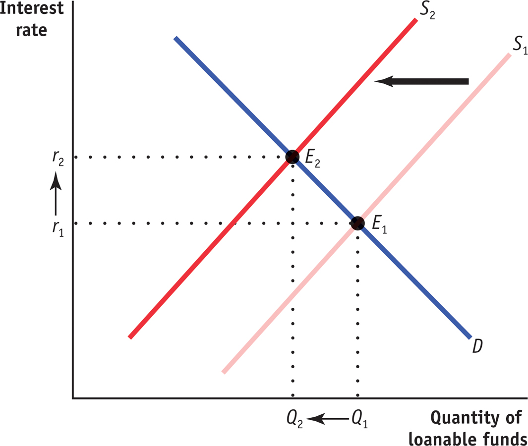
-
Explain what is wrong with the following statement: “Savings and investment spending may not be equal in the economy as a whole because when the interest rate rises, households will want to save more money than businesses will want to invest.”
We know from the loanable funds market that as the interest rate rises, households want to save more and consume less. But at the same time, an increase in the interest rate lowers the number of investment spending projects with returns at least as high as the interest rate. The statement “households will want to save more money than businesses will want to invest” cannot represent an equilibrium in the loanable funds market because it says that the quantity of loanable funds offered exceeds the quantity of loanable funds demanded. If that were to occur, the interest rate would fall to make the quantity of loanable funds offered equal to the quantity of loanable funds demanded.Suppose that expected inflation rises from 3% to 6%.
-
a. How will the real interest rate be affected by this change?
The real interest rate will not change. According to the Fisher effect, an increase in expected inflation drives up the nominal interest rate, leaving the real interest rate unchanged. -
b. How will the nominal interest rate be affected by this change?
The nominal interest rate will rise by 3%. Each additional percentage point of expected inflation drives up the nominal interest rate by 1 percentage point. -
c. What will happen to the equilibrium quantity of loanable funds?
As long as inflation is expected, it does not affect the equilibrium quantity of loanable funds. Both the supply and demand curves for loanable funds are pushed upward, leaving the equilibrium quantity of loanable funds unchanged.
-
Multiple-
Question
If the interest rate falls, then the present value of any given project __________ and total investment spending will __________.
A. B. C. D. E. Question
The real interest rate equals the
A. B. C. D. E. Question
Which of the following will increase the demand for loanable funds?
A. B. C. D. E. Question
Which of the following will increase the supply of loanable funds?
A. B. C. D. E. Question
Both lenders and borrowers base their decisions on
A. B. C. D. E.
Critical-
Does each of the following affect either the supply or the demand for loanable funds, and if so, does the affected curve increase (shift to the right) or decrease (shift to the left)?
There is an increase in capital inflows into the economy.
This causes an increase (rightward shift) in the supply of loanable funds.Businesses are pessimistic about future business conditions.
This causes a decrease (leftward shift) in the demand for loanable funds.The government increases borrowing.
This causes an increase (rightward shift) in the demand for loanable funds.The private savings rate decreases.
This causes a decrease (leftward shift) in the supply of loanable funds.