1.2 61Consumption and Investment Spending

Johner Images/Alamy
WHAT YOU WILL LEARN
 The meaning of the aggregate consumption function, which shows how current disposable income affects consumer spending
 How expected future income and aggregate wealth affect consumer spending
 The determinants of investment spending
 Why investment spending is a leading indicator of the future state of the economy
Consumer Spending
Should you splurge on a restaurant meal or save money by eating at home? Should you buy a new car and, if so, how expensive a model? Should you redo that bathroom or live with it for another year? In the real world, households are constantly confronted with such choices—
But what determines how much consumers spend?
Current Disposable Income and Consumer Spending
The most important factor affecting a family’s consumer spending is its current disposable income—
The Bureau of Labor Statistics (BLS) collects annual data on family income and spending. Families are grouped by levels of before-
Figure 61-1 is a scatter diagram showing the relationship between household current disposable income and household consumer spending for American households by income group in 2012. For example, point A shows that in 2012 the middle fifth of the population had an average current disposable income of $46,777 and average spending of $43,004. The pattern of the dots slopes upward from left to right, making it clear that households with higher current disposable income had higher consumer spending.

It’s very useful to represent the relationship between an individual household’s current disposable income and its consumer spending with an equation. The consumption function is an equation showing how an individual household’s consumer spending varies with the household’s current disposable income. The simplest version of a consumption function is a linear equation:
The consumption function is an equation showing how an individual household’s consumer spending varies with the household’s current disposable income.
(61-
where lowercase letters indicate variables measured for an individual household.

In this equation, c is individual household consumer spending and yd is individual household current disposable income. Recall that MPC, the marginal propensity to consume, is the amount by which consumer spending rises if current disposable income rises by $1. Finally, a is a constant term—
Notice, by the way, that we’re using y for income. That’s standard practice in macroeconomics, even though income isn’t actually spelled “yncome.” The reason is that I is reserved for investment spending.
Recall that we expressed MPC as the ratio of a change in consumer spending to the change in current disposable income. We’ve rewritten it for an individual household as Equation 61-
(61-
Multiplying both sides of Equation 61-
(61-
Equation 25-
Figure 61-2 shows what Equation 61-

In reality, actual data never fit Equation 61-
c = $18,478 + 0.520 × yd

That is, the data suggest a marginal propensity to consume of approximately 0.52. This implies that the marginal propensity to save (MPS)—the amount of an additional $1 of disposable income that is saved—
It’s important to realize that Figure 61-3 shows a microeconomic relationship between the current disposable income of individual households and their spending on goods and services. However, macroeconomists assume that a similar relationship holds for the economy as a whole: that there is a relationship, called the aggregate consumption function, between aggregate current disposable income and aggregate consumer spending. We’ll assume that it has the same form as the household-
The aggregate consumption function is the relationship for the economy as a whole between aggregate current disposable income and aggregate consumer spending.
(61-
Here, C is aggregate consumer spending (called just “consumer spending”); YD is aggregate current disposable income (called, for simplicity, just “disposable income”); and A is aggregate autonomous consumer spending, the amount of consumer spending when YD equals zero. This is the relationship represented in Figure 61-4 by CF, analogous to cf in Figure 61-3.

Shifts of the Aggregate Consumption Function
The aggregate consumption function shows the relationship between disposable income and consumer spending for the economy as a whole, other things equal. When things other than disposable income change, the aggregate consumption function shifts. There are two principal causes of shifts of the aggregate consumption function: changes in expected future disposable income and changes in aggregate wealth.
Changes in Expected Future Disposable IncomeSuppose you land a really good, well-
Conversely, suppose you have a good job but learn that the company is planning to downsize your division, raising the possibility that you may lose your job and have to take a lower-
Both of these examples show how expectations about future disposable income can affect consumer spending. The two panels of Figure 61-4, which plot disposable income against consumer spending, show how changes in expected future disposable income affect the aggregate consumption function. In both panels, CF1 is the initial aggregate consumption function. Panel (a) shows the effect of good news: information that leads consumers to expect higher disposable income in the future than they did before. Consumers will now spend more at any given level of current disposable income, YD, corresponding to an increase in A, aggregate autonomous consumer spending, from A1 to A2. The effect is to shift the aggregate consumption function up, from CF1 to CF2.
Panel (b) shows the effect of bad news: information that leads consumers to expect lower disposable income in the future than they did before. Consumers will now spend less at any given level of current disposable income, YD, corresponding to a fall in A from A1 to A2. The effect is to shift the aggregate consumption function down, from CF1 to CF2.
Changes in Aggregate WealthImagine two individuals, Maria and Mark, both of whom expect to earn $30,000 this year. Suppose, however, that they have different histories. Maria has been working steadily for the past 10 years, owns her own home, and has $200,000 in the bank. Mark is the same age as Maria, but he has been in and out of work, hasn’t managed to buy a house, and has very little in savings. In this case, Maria has something that Mark doesn’t have: wealth. Even though they have the same disposable income, other things equal, you’d expect Maria to spend more on consumption than Mark. That is, wealth has an effect on consumer spending.
The effect of wealth on spending is emphasized by an influential economic model of how consumers make choices about spending versus saving called the life-

We won’t go into the details of the life-
Because wealth affects household consumer spending, changes in wealth across the economy can shift the aggregate consumption function. A rise in aggregate wealth—
Investment Spending
Although consumer spending is much larger than investment spending, booms and busts in investment spending tend to drive the business cycle. In fact, most recessions originate as a fall in investment spending. Figure 61-5 illustrates this point; it shows the annual percent change of investment spending and consumer spending in the United States, measured in real terms, during six recessions from 1973 to 2009. As you can see, swings in investment spending are much more dramatic than those in consumer spending. In addition, due to the multiplier process, economists believe that declines in consumer spending are usually the result of a process that begins with a slump in investment spending. Soon we’ll examine in more detail how a slump in investment spending generates a fall in consumer spending through the multiplier process.

Before we do that, however, let’s analyze the factors that determine investment spending, which are somewhat different from those that determine consumer spending. The most important ones are the interest rate and expected future real GDP.
Planned investment spending is the investment spending that businesses intend to undertake during a given period.
It’s also important to note that the level of investment spending businesses actually carry out is sometimes not the same level as planned investment spending, the investment spending that firms intend to undertake during a given period. Planned investment spending depends on three principal factors: the interest rate, the expected future level of real GDP, and the current level of production capacity. First, we’ll analyze the effect of the interest rate.
The Interest Rate and Investment Spending
Interest rates have their clearest effect on one particular form of investment spending: spending on residential construction—
Consider a potential home-

Interest rates also affect other forms of investment spending. Firms with investment spending projects will only go ahead with a project if they expect a rate of return higher than the cost of the funds they would have to borrow to finance that project. As the interest rate rises, fewer projects will pass that test, and as a result investment spending will be lower.
You might think that the trade-
So the trade-
So planned investment spending—
Expected Future Real GDP, Production Capacity, and Investment Spending
Suppose a firm has enough capacity to continue to produce the amount it is currently selling but doesn’t expect its sales to grow in the future. Then it will engage in investment spending only to replace existing equipment and structures that wear out or are rendered obsolete by new technologies. But if, instead, the firm expects its sales to grow rapidly in the future, it will find its existing production capacity insufficient for its future production needs. So the firm will undertake investment spending to meet those needs. This implies that, other things equal, firms will undertake more investment spending when they expect their sales to grow.
Now suppose that the firm currently has considerably more capacity than necessary to meet current production needs. Even if it expects sales to grow, it won’t have to undertake investment spending for a while—
If we put together the effects on investment spending of growth in expected future sales and the size of current production capacity, we can see one situation in which we can be reasonably sure that firms will undertake high levels of investment spending: when they expect sales to grow rapidly. In that case, even excess production capacity will soon be used up, leading firms to resume investment spending.
According to the accelerator principle, a higher growth rate of real GDP leads to higher planned investment spending, but a lower growth rate of real GDP leads to lower planned investment spending.
What is an indicator of high expected growth of future sales? It’s a high expected future growth rate of real GDP. A higher expected future growth rate of real GDP results in a higher level of planned investment spending, but a lower expected future growth rate of real GDP leads to lower planned investment spending. This relationship is summarized in a proposition known as the accelerator principle.
As we explain in the upcoming Economics in Action, when expectations of future real GDP growth turned negative, planned investment spending—
Inventories and Unplanned Investment Spending
Inventories are stocks of goods held to satisfy future sales.
Most firms maintain inventories, stocks of goods held to satisfy future sales. Firms hold inventories so they can quickly satisfy buyers—
A firm that increases its inventories is engaging in a form of investment spending. Suppose, for example, that the U.S. auto industry produces 800,000 cars per month but sells only 700,000. The remaining 100,000 cars are added to the inventory at auto company warehouses or car dealerships, ready to be sold in the future.
Inventory investment is the value of the change in total inventories held in the economy during a given period.
Inventory investment is the value of the change in total inventories held in the economy during a given period. Unlike other forms of investment spending, inventory investment can actually be negative. If, for example, the auto industry reduces its inventory over the course of a month, we say that it has engaged in negative inventory investment.
To understand inventory investment, think about a manager stocking the canned goods section of a supermarket. The manager tries to keep the store fully stocked so that shoppers can almost always find what they’re looking for. But the manager does not want the shelves too heavily stocked because shelf space is limited and products can spoil.

Unplanned inventory investment occurs when actual sales are more or less than businesses expected, leading to unplanned changes in inventories.
Similar considerations apply to many firms and typically lead them to manage their inventories carefully. However, sales fluctuate. And because firms cannot always accurately predict sales, they often find themselves holding more or less inventories than they had intended. These unintended swings inventories due to unforeseen changes in sales are called unplanned inventory investment. They represent investment spending, positive or negative, that occurred but was unplanned.
So in any given period, actual investment spending is equal to planned investment spending plus unplanned inventory investment. If we let IUnplanned represent unplanned inventory investment, IPlanned represent planned investment spending, and I represent actual investment spending, then the relationship among all three can be represented as:
Actual investment spending is the sum of planned investment spending and unplanned inventory investment.
(61-
To see how unplanned inventory investment can occur, let’s continue to focus on the auto industry and make the following assumptions. First, let’s assume that the industry must determine each month’s production volume in advance, before it knows the volume of actual sales. Second, let’s assume that it anticipates selling 800,000 cars next month and that it plans neither to add to nor subtract from existing inventories. In that case, it will produce 800,000 cars to match anticipated sales.
Now imagine that next month’s actual sales are less than expected, only 700,000 cars. As a result, the value of 100,000 cars will be added to investment spending as unplanned inventory investment.
The auto industry will, of course, eventually adjust to this slowdown in sales and the resulting unplanned inventory investment. It is likely that it will cut next month’s production volume in order to reduce inventories. In fact, economists who study macroeconomic variables in an attempt to determine the future path of the economy pay careful attention to changes in inventory levels. Rising inventories typically indicate positive unplanned inventory investment and a slowing economy, as sales are less than had been forecast. Falling inventories typically indicate negative unplanned inventory investment and a growing economy, as sales are greater than forecast.
INTEREST RATES AND THE U.S. HOUSING BOOM
The housing boom in the Ft. Myers metropolitan area, described at the beginning of this section, was part of a broader housing boom in the country as a whole. There is little question that this housing boom was caused, in the first instance, by low interest rates.
Figure 61-6 shows the interest rate on 30-

The low interest rates led to a large increase in residential investment spending, reflected in a surge of housing starts, shown in panel (b). This rise in investment spending drove an overall economic expansion, both through its direct effects and through the multiplier process.
Unfortunately, the housing boom eventually turned into too much of a good thing. By 2006, it was clear that the U.S. housing market was experiencing a bubble: people were buying housing based on unrealistic expectations about future price increases. When the bubble burst, housing—
61
Solutions appear at the back of the book.
Check Your Understanding
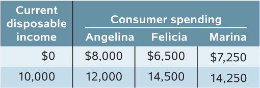
Suppose the economy consists of three people: Angelina, Felicia, and Marina. The table shows how their consumer spending varies as their current disposable income rises by $10,000.
-
a. Derive each individual’s consumption function, where MPC is calculated for a $10,000 change in current disposable income.
Angelina’s autonomous consumer spending is $8,000. When her current disposable income rises by $10,000, her consumer spending rises by $12,000 − $8,000 = $4,000. So her MPC is $4,000/$10,000 = 0.4 and her consumption function is c = $8,000 + 0.4 × yd. Felicia’s autonomous consumer spending is $6,500. When her current disposable income rises by $10,000, her consumer spending rises by $14,500 − $6,500 = $8,000. So her MPC is $8,000/$10,000 = 0.8 and her consumption function is c = $6,500 + 0.8 × yd. Marina’s autonomous consumer spending is $7,250. When her current disposable income rises by $10,000, her consumer spending rises by $14,250 − $7,250 = $7,000. So her MPC is $7,000/$10,000 = 0.7 and her consumption function is c = $7,250 + 0.7 × yd. -
b. Derive the aggregate consumption function.
The aggregate autonomous consumer spending in this economy is $8,000 + $6,500 + $7,250 = $21,750. A $30,000 increase in disposable income (3 × $10,000) leads to a $4,000 + $8,000 + $7,000 = $19,000 increase in consumer spending. So the economy-wide MPC is $19,000/$30,000 = 0.63 and the aggregate consumption function is C = $21,750 + 0.63 × YD.
-
Suppose that problems in the capital markets make consumers unable either to borrow or to put money aside for future use. What implication does this have for the effects of expected future disposable income on consumer spending?
If you expect your future disposable income to fall, you would like to save some of today’s disposable income to tide you over in the future. But you cannot do this if you cannot save. If you expect your future disposable income to rise, you would like to spend some of tomorrow’s higher income today. But you cannot do this if you cannot borrow. If you cannot save or borrow, your expected future disposable income will have no effect on your consumer spending today. In fact, your MPC must always equal 1: you must consume all your current disposable income today, and you will be unable to smooth your consumption over time.For each event, explain whether planned investment spending or unplanned inventory investment will change and in what direction.
-
a. an unexpected increase in consumer spending
An unexpected increase in consumer spending will result in a reduction in inventories as producers sell items from their inventories to satisfy this short-term increase in demand. This is negative unplanned inventory investment: it reduces the value of producers’ inventories. -
b. a sharp rise in the cost of business borrowing
A rise in the cost of borrowing is equivalent to a rise in the interest rate: fewer investment spending projects are now profitable to producers, whether they are financed through borrowing or retained earnings. As a result, producers will reduce the amount of planned investment spending. -
c. a sharp increase in the economy’s growth rate of real GDP
A sharp increase in the rate of real GDP growth leads to a higher level of planned investment spending by producers, according to the accelerator principle, as they increase production capacity to meet higher demand. -
d. an unanticipated fall in sales
As sales fall, producers sell less, and their inventories grow. This leads to positive unplanned inventory investment.
-
When consumer spending is sluggish an inventory overhang—a high level of unplanned inventory investment throughout the economy—
can make it difficult for the economy to recover quickly. Explain why an inventory overhang might, like the existence of too much production capacity, depress current economic activity. When consumer spending is sluggish, firms with excess production capacity will cut back on planned investment spending because they think their existing capacities are sufficient for expected future sales. Similarly, when consumer spending is sluggish and firms have a large amount of unplanned inventory investment, they are likely to cut back their production of output because they think their existing inventories are sufficient for expected future sales. So an inventory overhang is likely to depress current economic activity as firms cut back on their planned investment spending and on their output.
Multiple-
Question
Changes in which of the following lead to a shift of the aggregate consumption function?
I. expected future disposable income
II. aggregate wealth
III. current disposable incomeA. B. C. D. E. Question
The slope of a family’s consumption function is equal to
A. B. C. D. E. Question
Given the consumption function c = $16,000 + 0.5 yd, if individual household current disposable income is $20,000, individual household consumer spending will equal
A. B. C. D. E. Question
The level of planned investment spending is negatively related to the
A. B. C. D. E. Question
Actual investment spending in any period is equal to
A. B. C. D. E.
Critical-
List the three most important factors affecting planned investment spending. Explain how each is related to actual investment spending.
The three most important factors are these:
- The interest rate is the price (or opportunity cost) of investing, thus they are negatively related.
- Expected future real GDP—if a firm expects its sales to grow rapidly in the future, it will invest in expanded production capacity.
- Production capacity—if a firm finds its existing production capacity insufficient for its future production needs, it will undertake investment spending to meet those needs.