1.2 73The Money Market

WHAT YOU WILL LEARN
 What the money demand curve is
 Why the liquidity preference model determines the interest rate in the short run
The Demand for Money
In Module 69 we learned about the various types of monetary aggregates: M1, the most commonly used definition of the money supply, consists of currency in circulation (cash), plus checkable bank deposits, plus traveler’s checks; and M2, a broader definition of the money supply, consists of M1 plus deposits that can easily be transferred into checkable deposits. We also learned why people hold money—
The Opportunity Cost of Holding Money
Most economic decisions involve trade-
Individuals and firms find it useful to hold some of their assets in the form of money because of the convenience money provides: money can be used to make purchases directly, but other assets can’t. But there is a price to be paid for that convenience: money normally yields a lower rate of return than nonmonetary assets.
As an example of how convenience makes it worth incurring some opportunity costs, consider the fact that even today—

Even holding money in a checking account involves a trade-
So making sense of the demand for money is about understanding how individuals and firms trade off the benefit of holding cash—
Table 73-1 illustrates the opportunity cost of holding money in a specific month, June 2007. The first row shows the interest rate on one-
73-1
Selected Interest Rates, June 2007

Table 73-1 shows the opportunity cost of holding money at one point in time, but the opportunity cost of holding money changes when the overall level of interest rates changes. Specifically, when the overall level of interest rates falls, the opportunity cost of holding money falls, too.
Table 73-2 illustrates this point by showing how selected interest rates changed between June 2007 and June 2008, a period when the Federal Reserve was slashing rates in an (unsuccessful) effort to fight off a rapidly worsening recession.
73-2
Interest Rates and the Opportunity Cost of Holding Money

Short-
A comparison between interest rates in June 2007 and June 2008 illustrates what happens when the opportunity cost of holding money falls sharply. Between June 2007 and June 2008, the federal funds rate, which is the rate the Fed controls most directly, fell by 3.25 percentage points. The interest rate on one-
As short-
As a comparison of the two columns of Table 73-2 shows, the opportunity cost of holding money fell. The last two rows of Table 73-2 summarize this comparison: they give the differences between the interest rates on demand deposits and on currency and the interest rate on CDs. These differences—
The fact that the federal funds rate in Table 73-2 and the interest rate on one-
Conversely, investors will move their wealth into any short-
Long-
Table 73-2 contains only short-
Moreover, it’s short-
For the moment, however, let’s ignore the distinction between short-
The Money Demand Curve
Because the overall level of interest rates affects the opportunity cost of holding money, the quantity of money individuals and firms want to hold is, other things equal, negatively related to the interest rate.
In Figure 73-1, the horizontal axis shows the quantity of money demanded and the vertical axis shows the interest rate, r, which you can think of as a representative short-

The money demand curve shows the relationship between the interest rate and the quantity of money demanded.
The relationship between the interest rate and the quantity of money demanded by the public is illustrated by the money demand curve, MD, in Figure 73-1. The money demand curve slopes downward because, other things equal, a higher interest rate increases the opportunity cost of holding money, leading the public to reduce the quantity of money it demands. For example, if the interest rate is very low—
By contrast, if the interest rate is relatively high—
You might ask why we draw the money demand curve with the interest rate—
Stocks don’t fit that definition because there are significant transaction fees when you sell stock (which is why stock market investors are advised not to buy and sell too often). Real estate doesn’t fit the definition either because selling real estate involves even larger fees and can take a long time as well. So the relevant comparison is with assets that are “close to” money—
Shifts of the Money Demand Curve
A number of factors other than the interest rate affect the demand for money. When one of these factors changes, the money demand curve shifts. Figure 73-2 shows shifts of the money demand curve: an increase in the demand for money corresponds to a rightward shift of the MD curve, raising the quantity of money demanded at any given interest rate; a decrease in the demand for money corresponds to a leftward shift of the MD curve, reducing the quantity of money demanded at any given interest rate.

The most important factors causing the money demand curve to shift are changes in the aggregate price level, changes in real GDP, changes in credit markets and banking technology, and changes in institutions.
Changes in the Aggregate Price LevelAmericans keep a lot more cash in their wallets and funds in their checking accounts today than they did in the 1950s. One reason is that they have to if they want to be able to buy anything: almost everything costs more now than it did when you could get a burger, fries, and a drink at McDonald’s for 45 cents and a gallon of gasoline for 29 cents.
So, other things equal, higher prices increase the demand for money (a rightward shift of the MD curve), and lower prices decrease the demand for money (a leftward shift of the MD curve).
We can actually be more specific than this: other things equal, the demand for money is proportional to the price level. That is, if the aggregate price level rises by 20%, the quantity of money demanded at any given interest rate, such as r1 in Figure 73-2, also rises by 20%—the movement from M1 to M2. Why? Because if the price of everything rises by 20%, it takes 20% more money to buy the same basket of goods and services.
And if the aggregate price level falls by 20%, at any given interest rate the quantity of money demanded falls by 20%—shown by the movement from M1 to M3 at the interest rate r1. As we’ll see later, the fact that money demand is proportional to the price level has important implications for the long-
Changes in Real GDPHouseholds and firms hold money as a way to facilitate purchases of goods and services. The larger the quantity of goods and services they buy, the larger the quantity of money they will want to hold at any given interest rate. So an increase in real GDP—

Changes in Credit Markets and Banking TechnologyCredit cards are everywhere in American life today, but it wasn’t always so. The first credit card that allowed customers to carry a balance from month to month (called a “revolving balance”) was issued in 1959. Before then, people had to either pay for purchases in cash or pay off their balance every month.
The invention of revolving-
Changes in InstitutionsChanges in institutions can increase or decrease the demand for money. For example, until Regulation Q was eliminated in 1980, U.S. banks weren’t allowed to offer interest on checking accounts. So the interest you would forgo by holding funds in a checking account instead of an interest-
A YEN FOR CASH
Japan, say financial experts, is still a “cash society.” Visitors from the United States or Europe are surprised at how little use the Japanese make of credit cards and how much cash they carry around in their wallets. Yet Japan is an economically and technologically advanced country and, according to some measures, ahead of the United States in the use of telecommunications and information technology.

So why do the citizens of this economic powerhouse still do business the way Americans and Europeans did a generation ago? The answer highlights the factors affecting the demand for money.
One reason the Japanese use cash so much is that their institutions never made the switch to heavy reliance on plastic. For complex reasons, Japan’s retail sector is still dominated by small mom-
But there’s another reason the Japanese hold so much cash: there’s little opportunity cost to doing so. Short-
Money and Interest Rates
The Federal Open Market Committee decided today to lower its target for the federal funds rate 75 basis points to 2¼ percent.
Recent information indicates that the outlook for economic activity has weakened further. Growth in consumer spending has slowed and labor markets have softened. Financial markets remain under considerable stress, and the tightening of credit conditions and the deepening of the housing contraction are likely to weigh on economic growth over the next few quarters.
So read the beginning of a press release from the Federal Reserve issued on March 18, 2008. (A basis point is equal to 0.01 percentage point. So the statement implies that the Fed lowered the target from 3% to 2.25%.) Recall that the federal funds rate is the rate at which banks lend reserves to each other to meet the required reserve ratio.
As the statement implies, at each of its eight-
As we’ve already seen, other short-
How does the Fed go about achieving a target federal funds rate? And more to the point, how is the Fed able to affect interest rates at all?
The Equilibrium Interest Rate
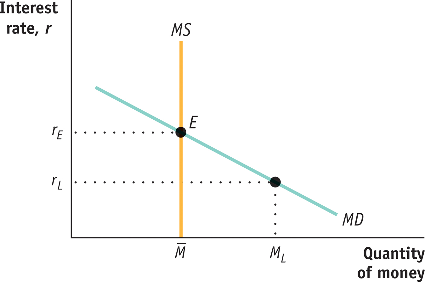
According to the liquidity preference model of the interest rate, the interest rate is determined by the supply and demand for money.
The money supply curve shows how the quantity of money supplied varies with the interest rate.
Remember that, for simplicity, we’re assuming there is only one interest rate paid on nonmonetary financial assets, both in the short run and in the long run. To understand how the interest rate is determined, consider Figure 73-3, which illustrates the liquidity preference model of the interest rate; this model says that the interest rate is determined by the supply and demand for money in the market for money. Figure 73-3 combines the money demand curve, MD, with the money supply curve, MS, which shows how the quantity of money supplied by the Federal Reserve varies with the interest rate.

 . The money market is in equilibrium at the interest rate rE: the quantity of money demanded by the public is equal to , the quantity of money supplied.
At a point such as L, the interest rate, rL, is below rE and the corresponding quantity of money demanded, ML, exceeds the money supply,
. In an attempt to shift their wealth out of nonmoney interest-. In an attempt to shift out of money holdings into nonmoney interest-In the previous module we learned how the Federal Reserve can increase or decrease the money supply: it usually does this through open-
Let’s assume for simplicity that the Fed, using one or more of these methods, simply chooses the level of the money supply that it believes will achieve its interest rate target. Then the money supply curve is a vertical line, MS in Figure 73-3, with a horizontal intercept corresponding to the money supply chosen by the Fed, . The money market equilibrium is at E, where MS and MD cross. At this point the quantity of money demanded equals the money supply, , leading to an equilibrium interest rate of rE.
To understand why rE is the equilibrium interest rate, consider what happens if the money market is at a point like L, where the interest rate, rL, is below rE. At rL the public wants to hold the quantity of money ML, an amount larger than the actual money supply, This means that at point L, the public wants to shift some of its wealth out of interest-
This has two implications. One is that the quantity of money demanded is more than the quantity of money supplied. The other is that the quantity of interest-. That is, the interest rate will rise until it is equal to rE.
Now consider what happens if the money market is at a point such as H in Figure 73-3, where the interest rate rH is above rE. In that case the quantity of money demanded, MH, is less than the quantity of money supplied, . Correspondingly, the quantity of interest-. Again, the interest rate will end up at rE.
Two Models of Interest Rates?
You might have noticed that this is the second time we have discussed the determination of the interest rate. In an earlier module, we studied the loanable funds model of the interest rate; according to that model, the interest rate is determined by the equalization of the supply of funds from lenders and the demand for funds by borrowers in the market for loanable funds. But here we have described a seemingly different model in which the interest rate is determined by the equalization of the supply and demand for money in the money market.
Which of these models is correct? The answer is both, depending on context. The loanable funds model is focused on the interest rate in the long run. The money market model, however, focuses on the interest rate in the short run.
73
Solutions appear at the back of the book.
Check Your Understanding
Explain how each of the following would affect the quantity of money demanded, and indicate whether each change would cause a movement along the money demand curve or a shift of the money demand curve.
-
a. Short-
term interest rates rise from 5% to 30%. By increasing the opportunity cost of holding money, a high interest rate reduces the quantity of money demanded. This is a movement up and to the left along the money demand curve. -
b. All prices fall by 10%.
A 10% fall in prices reduces the quantity of money demanded at any given interest rate, shifting the money demand curve leftward. -
c. New wireless technology automatically charges supermarket purchases to credit cards, eliminating the need to stop at the cash register.
This technological change reduces the quantity of money demanded at any given interest rate, so it shifts the money demand curve leftward. -
d. In order to avoid paying taxes, a vast underground economy develops in which workers are paid their wages in cash rather than with checks.
Payments in cash require employers to hold more money, increasing the quantity of money demanded at any given interest rate. So it shifts the money demand curve rightward.
-
Will each of the following increase the opportunity cost of holding cash, reduce it, or have no effect on it? Explain your answers.
-
a. Merchants charge a 1% processing fee on debit/credit card transactions for purchases of less than $50.
A 1% processing fee on debit/credit card transactions for purchases less than $50 reduces the opportunity cost of holding cash because consumers will save money by paying with cash. -
b. To attract more deposits, banks raise the interest paid on six-
month CDs. An increase in the interest paid on six-month CDs raises the opportunity cost of holding cash because holding cash requires forgoing the higher interest paid. -
c. Real estate prices fall significantly.
A fall in real estate prices has no effect on the opportunity cost or benefit of holding cash because real estate is an illiquid asset and therefore isn’t relevant in the decision of how much cash to hold. Also, real estate transactions are generally not carried out using cash. -
d. The cost of food rises significantly.
Because many purchases of food are made in cash, a significant increase in the cost of food reduces the opportunity cost of holding cash.
-
Multiple-
Question
A change in which of the following will shift the money demand curve?
I. the aggregate price level
II. real GDP
III. the interest rateA. B. C. D. E. Question
Which of the following will decrease the demand for money?
A. B. C. D. E. Question
What will happen to the money supply and the equilibrium interest rate if the Federal Reserve sells Treasury securities?
Money supplyEquilibrium interest rateA. B. C. D. E. Question
Which of the following is true regarding short-
term and long- term interest rates? A. B. C. D. E. Question
The quantity of money demanded rises (that is, there is a movement along the money demand curve) when
A. B. C. D. E.
Critical-
Draw a graph showing equilibrium in the money market. Select an interest rate below the equilibrium interest rate and explain what occurs in the market at that interest rate and how the market will eventually return to equilibrium.