We’ve just seen that in the short run a fall in the aggregate price level leads to a decline in the quantity of aggregate output supplied because nominal wages are sticky in the short run. But, as we mentioned earlier, contracts and informal agreements are renegotiated in the long run. So in the long run, nominal wages—like the aggregate price level—are flexible, not sticky. This fact greatly alters the long-run relationship between the aggregate price level and aggregate supply. In fact, in the long run the aggregate price level has no effect on the quantity of aggregate output supplied.

To see why, let’s conduct a thought experiment. Imagine that you could wave a magic wand—or maybe a magic bar-code scanner—and cut all prices in the economy in half at the same time. By “all prices” we mean the prices of all inputs, including nominal wages, as well as the prices of final goods and services. What would happen to aggregate output, given that the aggregate price level has been halved and all input prices, including nominal wages, have been halved?

The answer is: nothing. Consider Equation 12-2 again: each producer would receive a lower price for its product, but costs would fall by the same proportion. As a result, every unit of output profitable to produce before the change in prices would still be profitable to produce after the change in prices. So a halving of all prices in the economy has no effect on the economy’s aggregate output. In other words, changes in the aggregate price level now have no effect on the quantity of aggregate output supplied.

In reality, of course, no one can change all prices by the same proportion at the same time. But now, we’ll consider the long run, the period of time over which all prices are fully flexible. In the long run, inflation or deflation has the same effect as someone changing all prices by the same proportion. As a result, changes in the aggregate price level do not change the quantity of aggregate output supplied in the long run. That’s because changes in the aggregate price level will, in the long run, be accompanied by equal proportional changes in all input prices, including nominal wages.

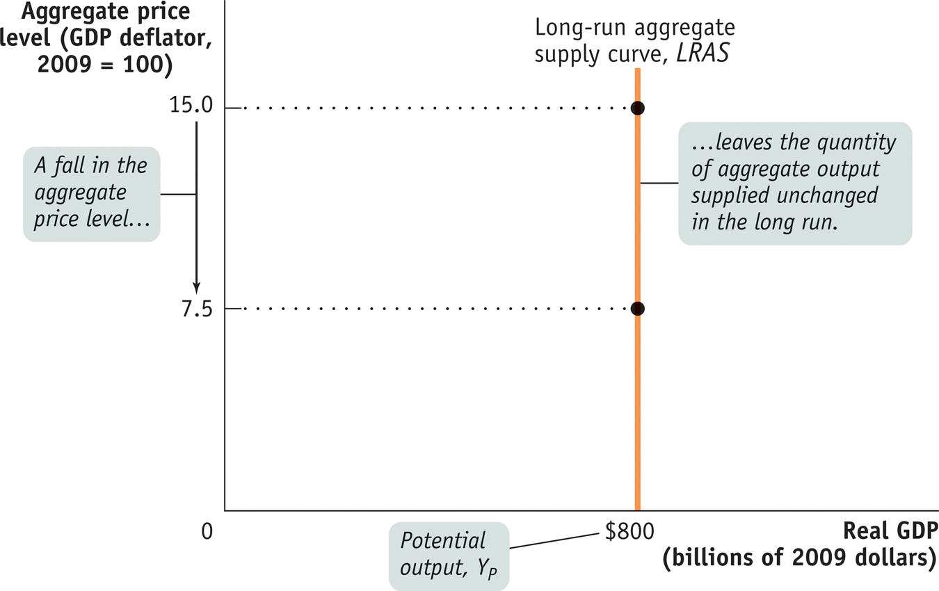
The long-run aggregate supply curve, illustrated in Figure 12-7 by the curve LRAS, shows the relationship between the aggregate price level and the quantity of aggregate output supplied that would exist if all prices, including nominal wages, were fully flexible. The long-run aggregate supply curve is vertical because changes in the aggregate price level have no effect on aggregate output in the long run. At an aggregate price level of 15.0, the quantity of aggregate output supplied is $800 billion in 2009 dollars. If the aggregate price level falls by 50% to 7.5, the quantity of aggregate output supplied is unchanged in the long run at $800 billion in 2009 dollars.

It’s important to understand not only that the LRAS curve is vertical but also that its position along the horizontal axis represents a significant measure. The horizontal intercept in Figure 12-7, where LRAS touches the horizontal axis ($800 billion in 2009 dollars), is the economy’s potential output, Y_P: the level of real GDP the economy would produce if all prices, including nominal wages, were fully flexible.

In reality, the actual level of real GDP is almost always either above or below potential output. We’ll see why later in this chapter, when we discuss the AD–AS model. Still, an economy’s potential output is an important number because it defines the trend around which actual aggregate output fluctuates from year to year.

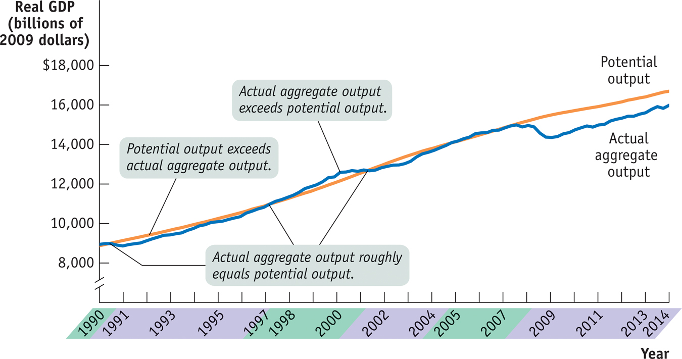
In the United States, the Congressional Budget Office, or CBO, estimates annual potential output for the purpose of federal budget analysis. In Figure 12-8, the CBO’s estimates of U.S. potential output from 1990 to 2014 are represented by the orange line and the actual values of U.S. real GDP over the same period are represented by the blue line. Years shaded purple on the horizontal axis correspond to periods in which actual aggregate output fell short of potential output, years shaded green to periods in which actual aggregate output exceeded potential output.

As you can see, U.S. potential output has risen steadily over time—implying a series of rightward shifts of the LRAS curve. What has caused these rightward shifts? The answer lies in the factors related to long-run growth that we discussed in Chapter 9, such as increases in physical capital and human capital as well as technological progress. Over the long run, as the size of the labor force and the productivity of labor both rise, the level of real GDP that the economy is capable of producing also rises. Indeed, one way to think about long-run economic growth is that it is the growth in the economy’s potential output. We generally think of the long-run aggregate supply curve as shifting to the right over time as an economy experiences long-run growth.