From the Short Run to the Long Run
As you can see in Figure 12-8, the economy normally produces more or less than potential output: actual aggregate output was below potential output in the early 1990s, above potential output in the late 1990s, below potential output for most of the 2000s, and significantly below potential output after the recession of 2007–
The first step to answering these questions is to understand that the economy is always in one of only two states with respect to the short-
PITFALLS: ARE WE THERE YET? WHAT THE LONG RUN REALLY MEANS
ARE WE THERE YET? WHAT THE LONG RUN REALLY MEANS
We’ve used the term long run in two different contexts. In an earlier chapter we focused on long-
Because the economy always tends to return to potential output in the long run, actual aggregate output fluctuates around potential output, rarely getting too far from it. As a result, the economy’s rate of growth over long periods of time—
Figure 12-9 illustrates how this process works. In both panels LRAS is the long-
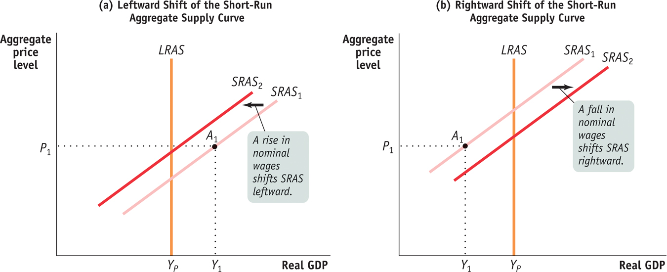
In panel (b), the initial production point, A1, corresponds to an aggregate output level, Y1, that is lower than potential output, YP. Producing an aggregate output level (such as Y1) that is lower than potential output (YP) is possible only because nominal wages haven’t yet fully adjusted downward. Until this downward adjustment occurs, producers are earning low (or negative) profits and producing a low level of output. An aggregate output level lower than potential output means high unemployment. Because workers are abundant and jobs are scarce, nominal wages will fall over time, shifting the short-
We’ll see shortly that these shifts of the short-
!worldview! ECONOMICS in Action: Sticky Wages in the Great Recession
Sticky Wages in the Great Recession
We’ve asserted that the aggregate supply curve is upward-
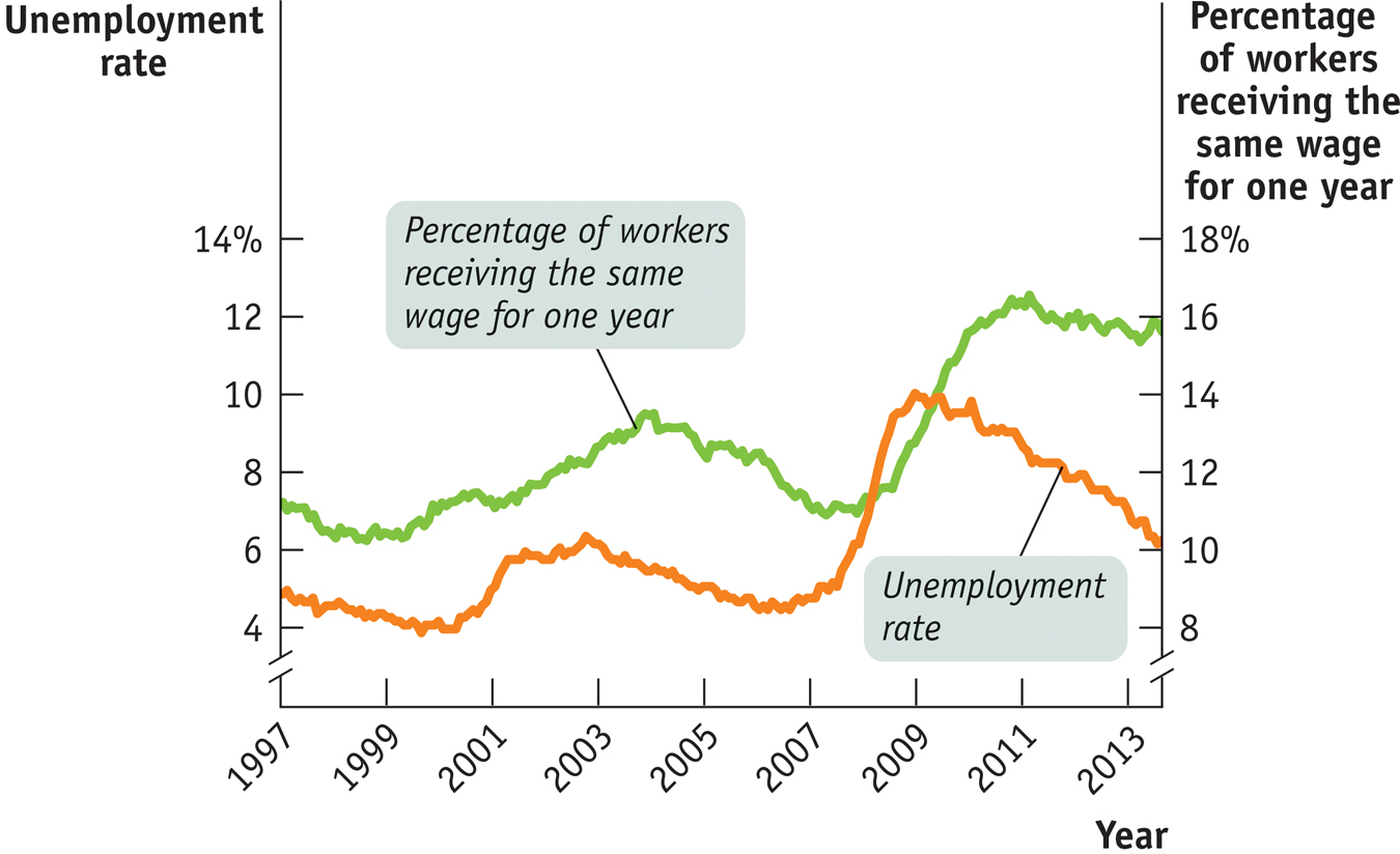
The answer is that we can look at what happens to wages at times when we might have expected to see many workers facing wage cuts because similar workers are unemployed and would be willing to work for less. If wages are sticky, what we would expect to find at such times is that many workers’ wages don’t change at all: there’s no reason for employers to give them a raise, but because wages are sticky, they don’t face cuts either.
And that is exactly what you find during and after the Great Recession of 2007–
Similar results can be found in European nations facing high unemployment, such as Spain. The Great Recession provided strong confirmation that wages are indeed sticky.
When unemployment soared in the face of the economic slump following the 2008 financial crisis, you might have expected to see widespread wage cuts. But employers are reluctant to cut wages. So what we saw instead was a sharp rise in the number of workers whose wages were flat—
Quick Review
The aggregate supply curve illustrates the relationship between the aggregate price level and the quantity of aggregate output supplied.
The short-
run aggregate supply curve is upward sloping: a higher aggregate price level leads to higher aggregate output given that nominal wages are sticky.Changes in commodity prices, nominal wages, and productivity shift the short-
run aggregate supply curve. In the long run, all prices are flexible, and changes in the aggregate price level have no effect on aggregate output. The long-
run aggregate supply curve is vertical at potential output.If actual aggregate output exceeds potential output, nominal wages eventually rise and the short-
run aggregate supply curve shifts leftward. If potential output exceeds actual aggregate output, nominal wages eventually fall and the short- run aggregate supply curve shifts rightward.
12-2
Question 12.2
Determine the effect on short-
run aggregate supply of each of the following events. Explain whether it represents a movement along the SRAS curve or a shift of the SRAS curve. A rise in the consumer price index (CPI) leads producers to increase output.
A fall in the price of oil leads producers to increase output.
A rise in legally mandated retirement benefits paid to workers leads producers to reduce output.
Question 12.3
Suppose the economy is initially at potential output and the quantity of aggregate output supplied increases. What information would you need to determine whether this was due to a movement along the SRAS curve or a shift of the LRAS curve?
Solutions appear at back of book.